Two signals are recorded from each of forty people. You want to know how strongly they are coupled, at which frequencies, and whether the coupling differs between two groups.
The usual answer is a two-stage pipeline: estimate each person’s coherence, then test the estimates. This article shows what that costs, on data whose truth is known, and what one hierarchical fit gives instead.
Why the usual answer is wrong
Coherence from n segments is biased upward by roughly
(1 - C)^2 / n. At a true coherence of zero the estimate has
mean exactly 1/n, so a person with 4 segments reads 0.25
when the truth is nothing at all.
Two things are usually done about it, and both fail.
Averaging over people does not help. The mean of forty biased numbers carries the same bias, because the bias is in each number rather than in the spread.
one_unit <- function(n, coh, phase, la = 0, lb = 0) {
  a <- exp(la); b <- exp(lb); cm <- b * sqrt(coh / (1 - coh))
  z1 <- complex(real = rnorm(n, 0, sqrt(0.5)), imaginary = rnorm(n, 0, sqrt(0.5)))
  z2 <- complex(real = rnorm(n, 0, sqrt(0.5)), imaginary = rnorm(n, 0, sqrt(0.5)))
  d1 <- a * z1
  d2 <- cm * complex(modulus = 1, argument = -phase) * z1 + b * z2
  cr <- sum(d1 * Conj(d2))
  c(w11 = sum(Mod(d1)^2), w22 = sum(Mod(d2)^2),
    w12r = Re(cr), w12i = Im(cr), n = n)
}
naive_mean <- function(N, n, coh) {
  m <- t(replicate(N, one_unit(n, coh, 0.5)))
  mean((m[, "w12r"]^2 + m[, "w12i"]^2) / (m[, "w11"] * m[, "w22"]))
}
round(sapply(c(2, 4, 8, 16, 32), function(n) naive_mean(400, n, 0.2)), 3)
#> [1] 0.572 0.393 0.277 0.244 0.229
The truth is 0.2 in every one of those. Four segments reads about 0.39.
Concatenating everyone’s segments is worse. Pooling is valid only if every person has the same spectral matrix. Once phase varies between people, the cross terms cancel:
N <- 40; n <- 8
u <- t(replicate(N, one_unit(n, 0.5, rnorm(1, 0.8, 0.8))))
pooled <- (sum(u[, "w12r"])^2 + sum(u[, "w12i"])^2) /
  (sum(u[, "w11"]) * sum(u[, "w22"]))
c(truth = 0.5, naive_mean = mean((u[, "w12r"]^2 + u[, "w12i"]^2) /
                                   (u[, "w11"] * u[, "w22"])),
  pooled = pooled)
#>      truth naive_mean     pooled
#>  0.5000000  0.5668223  0.2977686
Pooling reads far below the truth, and unlike the naive bias it does not shrink with more segments, because it is cancellation rather than variance.
Where this package does not help
The bias is roughly (1 - C)^2 / n, so it vanishes as the
coupling gets strong. Here is the naive bias at 4 segments across three
true coherences:
round(sapply(c(0.2, 0.5, 0.9), function(C) naive_mean(2000, 4, C)) -
        c(0.2, 0.5, 0.9), 3)
#> [1] 0.175 0.085 0.004
At a true coherence of 0.9 the bias is a few thousandths against 0.175 at 0.2. There is nothing to correct up there, and this package buys you nothing for it.
The whole argument lives at low to moderate coherence, which is also where most real cortico-muscular and cortico-cortical couplings sit. If your coherences are all above about 0.8, fit whatever is convenient and report it; the reason to come here is a hierarchical question, an interval you trust, or a group comparison, not the bias.
The model
The pair’s periodogram at one frequency is complex Wishart about the
spectral matrix. cross_wishart() is that likelihood,
parameterized so its four distributional parameters are the two channel
powers, the coherence and the phase. Each takes a formula, so a random
effect on coherence is written the way any random effect is written.
xs <- as.data.frame(t(replicate(N, one_unit(n, 0.5, rnorm(1, 0.8, 0.8),
                                            la = rnorm(1, 0, 0.3),
                                            lb = rnorm(1, 0, 0.3)))))
xs$id <- factor(seq_len(N))
head(xs, 3)
#>         w11       w22      w12r      w12i n id
#> 1 11.883109  6.461627 0.2445355  6.129594 8  1
#> 2  7.473119 29.736050 5.2062126 12.518727 8  2
#> 3  5.495194  7.463301 2.3805728  3.623912 8  3
fit <- frm(bf(w11 | vreal(w22, w12r, w12i) + vint(n) ~ 1 + (1 | id),
              pow2 ~ 1 + (1 | id),
              coh ~ 1 + (1 | id),
              phase ~ 1 + (1 | id)),
           family = cross_wishart(), data = xs)
#> Boundary (singular) fit: sd_id__coh_Intercept is at zero. The likelihood does not change as it moves further that way, so it has no standard error (NaN in summary(), vcov() and confint()); the other standard errors are kept. lme4 reports such a fit as singular; diagnose() lists the components at the boundary
frm_coherence(fit, newdata = xs[1, ], re_formula = NA)
#>   .estimate       .se    .lower    .upper       .eta
#> 1 0.4695287 0.1226127 0.4103901 0.5295356 -0.1220363
The interval is a Wald interval on the logit scale pushed through
plogis(), so it cannot leave (0, 1) however
close to a boundary the estimate sits. That boundary is where the
arithmetic has to be careful: plogis(eta) is exactly 1 in
double precision above about eta = 36.7, so the density
never forms 1 - C by subtraction. It asks core for
log(1 - C) with frmtmb::dpar_log1m(), which
reads the linear predictor core keeps beside each parameter and is exact
to eta = 709. A draft of this package did subtract, and
returned NaN above eta = 36.7 and a confidence
interval of width zero for two signals that differed only by 1e-5 of
noise.
Put a random effect on every parameter, not only on coherence
The two channel powers are incidental parameters: two free numbers per person that gain no information as people are added. Left free, they starve the coherence variance component, which collapses to zero without a warning; the fit converges and its interval covers 62 percent of the time instead of 95.
| what carries a random effect | bias at n = 4 | 95% coverage |
|---|---|---|
| coherence and phase only, powers free per person | +0.068 | 0.622 |
| all four parameters | +0.008 | 0.912 |
Measured over 150 replicates, 40 people;
dev/xspec-findings.md in the repository has the full table.
It is the failure that looks most like success.
A contrast needs the grouping it varies within
Two conditions measured in the same people is the other design where
an interval quietly comes back the wrong width. (1 | id)
does not fix it: a subject effect shifts both of that subject’s
conditions together, so it cancels out of their difference. The term
that carries a within-subject contrast is
(1 | id:cond).
coh ~ cond + s(freq, by = cond) + (1 | id) + (1 | id:cond)Over 148 replicates of 40 people by 2 conditions by 60 frequencies,
with a true contrast of 0.5 on the logit scale, sd(id) 0.35
and sd(id:cond) 0.20:
| coherence model | 95% coverage | interval width |
|---|---|---|
| condition, smooth and a subject effect | 0.527 | 0.37 |
| the same plus a subject-by-condition effect | 0.953 | 1.00 |
Both models put the contrast in the same place, within 0.0036 of each
other on the same data. The one without (1 | id:cond)
reports an interval 2.7 times too narrow, and on 63 of the 148
replicates it missed the truth where the correct model covered. It never
covered where the correct model missed. Width is the whole difference:
with the component absent from the truth the two models agree to a
median width ratio of 1.000, and the interval the shorter model reports
on data that HAS the component, 0.070, is the interval the correct model
reports on data that does not, 0.072.
The direction depends on which term is missing. Keeping
(1 | id:cond) and dropping (1 | id) gives an
interval 1.9 times too WIDE, because the subject variance is then forced
into the crossed term. So the rule is neither more random effects nor
fewer: a within-subject contrast needs both terms, the subject one for
the intercept and the crossed one for the contrast.
Dropping the random effects entirely is a different thing
A model with no random effect at all, coh ~ cond or
coh ~ cond + s(freq, by = cond), is not making a small
version of the same mistake. Its interval is narrow for the same reason,
but its estimate has also moved, by -0.0197 and -0.0133 over those 148
replicates, and that movement is not an error. A contrast on a logit
scale is not collapsible: leave variance out of the linear predictor and
the fit is consistent for the population-averaged
contrast, which is smaller than the subject-level one by about
1 / sqrt(1 + 0.346 V) with V the variance left
out. From the simulation’s own constants, with nothing fitted, that
factor predicts -0.0196 and -0.0135.
So decide which contrast you want. If it is the subject-level one, model the variance; a wider interval does not convert one into the other.
From signals to rows
frm_cross_spectrum() does the data preparation,
including the parts that are easy to get wrong and impossible to notice:
it drops frequency zero and the Nyquist frequency, whose coefficients
are real rather than complex, and it counts the degrees of freedom
honestly.
sfreq <- 128
src <- as.numeric(filter(rnorm(4096), 0.9, method = "recursive"))
a <- src + rnorm(4096, 0, 0.5)
b <- 0.9 * src + rnorm(4096, 0, 2)
sp <- frm_cross_spectrum(a, b, sfreq = sfreq, segments = 16)
head(sp, 3)
#>   freq       w11       w22      w12r      w12i  n
#> 1  0.5 1678.5668 1453.5994 1522.6362  65.39112 16
#> 2  1.0  927.8641  764.1049  809.0603 -38.48858 16
#> 3  1.5  641.8278  554.8955  547.1008  10.59337 16
Segments, sine tapers and frequency smoothing all buy real degrees of
freedom, and all three deliver the nominal count to within 2 percent on
white noise. tapers and smooth may not both
exceed 1: they widen the same spectral window, so their product is not
the count. Four tapers smoothed over four bins buys 5.8 draws, not
16.
window = "hann" is the fourth option and the one that
buys nothing. Use it where leakage is the larger error, which is a steep
spectrum: a raised cosine leaves the draw count alone (8.02 measured
against a nominal 8) and cannot be combined with tapers or
smooth, for the reason above.
What a window and a taper both cost is the independence of the rows,
which n does not describe. At the default eight segments
the correlation of adjacent frequencies is 0.40 with a Hann window and
-0.01 without, and 0.75 at tapers = 4. As a variance
inflation factor for a mean over the rows that is 1.8 for the window,
4.1 for four tapers and 8.0 for eight, so an s(freq) band
fitted on a tapered frame is optimistic. The per-row n is
right in all of them; it is a different quantity.
A recording with artifact-rejected spans in it is one call.
NA marks a sample the pair does not have; the record is cut
there and segments are laid inside the clean spans, so no transform
crosses a gap and the answer is exactly the sum of the clean pieces.
n then reports the segments the record supplied rather than
the number asked for, which is the count every standard error downstream
is formed from.
A trial-based recording is a list of epochs, and after artifact
rejection they are rarely of one length. Pass the two signals as two
lists, one element per epoch, with group naming the unit
each epoch belongs to. The epochs of one unit are read as the clean
spans of one record: one segment length for the unit, segments laid
inside each epoch, and no transform crossing from one epoch into the
next.
len <- c(900, 1300, 700, 1100, 1000, 800)
ea <- lapply(len, function(m) rnorm(m))
eb <- lapply(ea, function(v) 0.7 * v + rnorm(length(v)))
ep <- frm_cross_spectrum(ea, eb, sfreq = sfreq, segments = 8,
                         group = rep(c("s01", "s02"), each = 3))
table(ep$id, ep$n)
#>
#>         6   7
#>   s01 180   0
#>   s02   0 180
Each subject gets one frequency grid and one n. A vector
pair with a group of one label per sample, the spelling
frmtmb::frm_periodogram() takes, is the same thing when
each label is one epoch.
The one trap
The likelihood couples the powers and the coherence. A power formula too simple for the spectrum does not merely leave the powers wrong; it reweights the rows each coherence parameter pools and moves the coherence with them.
sp$band <- factor(ifelse(sp$freq < 32, "low", "high"), c("low", "high"))
flat <- frm(bf(w11 | vreal(w22, w12r, w12i) + vint(n) ~ 1,
               pow2 ~ 1, coh ~ band, phase ~ 1),
            family = cross_wishart(), data = sp)
Nothing warned about the thing that matters. The fit may report a
large maximum absolute gradient, which is about the optimizer and not
about this; core raises it on Gamma(link = "log") fits of
the same response too, and it is seed dependent. What it does NOT say is
that the coherence you are about to read has been displaced.
There is no automatic check for it, and that is deliberate. A draft
of this package warned from a fit_check hook that measured
the spread of the power residuals, and that statistic turned out not to
track the coherence displacement: it stayed silent at a 2.7-fold power
spread where the reported coherence was already nearly double the truth,
and it fired at a ratio of 20.5 on a correctly specified model whose
coherences were right. A check that punishes correct models teaches
people to ignore it, so it was withdrawn.
Compare AIC instead. Fit the powers with and without a frequency term and keep the one AIC prefers:
good <- frm(bf(w11 | vreal(w22, w12r, w12i) + vint(n) ~ s(freq, k = 8),
               pow2 ~ s(freq, k = 8), coh ~ band, phase ~ 1),
            family = cross_wishart(), data = sp)
nd <- data.frame(band = factor(c("low", "high"), c("low", "high")),
                 freq = c(16, 48))
rbind(flat = frm_coherence(flat, newdata = nd)$.estimate,
      good = frm_coherence(good, newdata = nd)$.estimate)
#>           [,1]       [,2]
#> flat 0.4579340 0.40876097
#> good 0.3591104 0.04314382
c(AIC_flat = AIC(flat), AIC_good = AIC(good), delta = AIC(flat) - AIC(good))
#> AIC_flat AIC_good    delta
#> 8490.902 4089.772 4401.130
The shared source is low-pass, so the low band really is the coherent one. The flat fit calls the two bands nearly equal; the well specified one separates them, and AIC prefers it by thousands.
The comparison works where the withdrawn hook did not. On a two-band
design at n = 8 with true coherences 0.35 and 0.05, varying
how much the power slopes across the record:
| power spread | flat powers report | correct powers report | delta AIC |
|---|---|---|---|
| 1.6x | 0.295, 0.083 | 0.330, 0.068 | 80 |
| 2.7x | 0.268, 0.078 | 0.342, 0.041 | 487 |
| 7.3x | 0.240, 0.206 | 0.342, 0.047 | 1849 |
| 19.6x | 0.229, 0.458 | 0.341, 0.052 | 3716 |
| 385x | 0.222, 0.875 | 0.342, 0.059 | 11518 |
AIC rejects the flat model by 80 or more even at the mildest spread, and the correct model recovers 0.35 and 0.05 throughout. Model the powers before reading any coherence.
A coherence spectrum
Coherence that varies with frequency is a smooth on coh.
It cannot leave (0, 1) at any point on the smooth, because
the logit link is the positive definiteness constraint rather than a
convenience.
spec <- frm(bf(w11 | vreal(w22, w12r, w12i) + vint(n) ~ s(freq, k = 10),
               pow2 ~ s(freq, k = 10), coh ~ s(freq, k = 10), phase ~ 1),
            family = cross_wishart(), data = sp)
co <- frm_coherence(spec)
range(co$.lower)
#> [1] 0.009043084 0.884928064
range(co$.upper)
#> [1] 0.05689554 0.93557526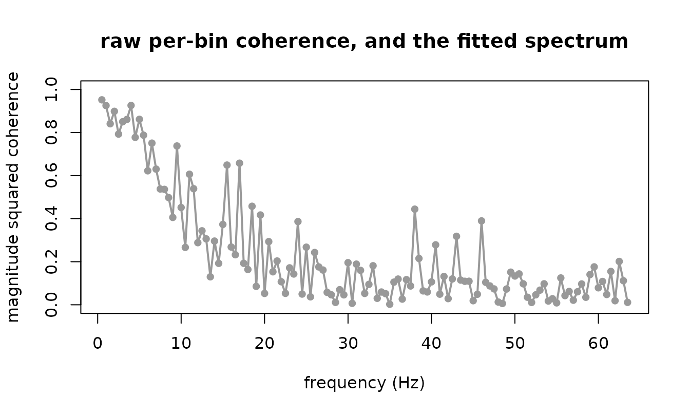
The grey points are each bin’s own coherence, every one of them
biased upward by about 1/16; the line is the fitted
spectrum, which borrows strength across frequency and does not have to
be.
Many channels: every pair in one model
cross_wishart() models one pair. A recording with four
channels has six pairs, and the usual analysis fits each pair on its own
and then corrects six p-values for multiplicity.
frm_cross_pairs() stacks the pairs instead, with a
pair factor, so that one model holds all of them.
n4 <- 4096
s4 <- rnorm(n4)
X <- cbind(Fz = s4 + rnorm(n4), Cz = 0.8 * s4 + rnorm(n4),
           Pz = 0.5 * s4 + rnorm(n4), Oz = 0.25 * s4 + rnorm(n4))
xp <- frm_cross_pairs(X, sfreq = sfreq, segments = 16)
levels(xp$pair)
#> [1] "Fz-Cz" "Fz-Pz" "Fz-Oz" "Cz-Pz" "Cz-Oz" "Pz-Oz"
(1 | pair) on coh is the
multiple-comparison story. Each pair gets its own coherence, drawn
toward the pairs’ common level by as much as the data say the pairs
differ, so a pair that stands out does so against the other pairs and
not against a correction applied afterwards. The powers and the phase
belong to the pair, so they are fixed effects of it.
pf <- frm(bf(w11 | vreal(w22, w12r, w12i) + vint(n) ~ 0 + pair,
             pow2 ~ 0 + pair, coh ~ 1 + (1 | pair), phase ~ 0 + pair),
          family = cross_wishart(), data = xp)
nd <- data.frame(pair = factor(levels(xp$pair), levels = levels(xp$pair)))
cbind(nd, round(frm_coherence(pf, newdata = nd), 3))
#>    pair .estimate   .se .lower .upper   .eta
#> 1 Fz-Cz     0.196 0.071  0.175  0.219 -1.413
#> 2 Fz-Pz     0.090 0.104  0.075  0.108 -2.312
#> 3 Fz-Oz     0.030 0.179  0.021  0.042 -3.477
#> 4 Cz-Pz     0.079 0.111  0.065  0.097 -2.454
#> 5 Cz-Oz     0.023 0.205  0.015  0.033 -3.770
#> 6 Pz-Oz     0.010 0.299  0.006  0.018 -4.566
A coherence that varies with frequency differently in each pair is
s(freq, by = pair), with pair also a fixed
effect so that each smooth has its own level;
frm_coherence() then gives each pair’s spectrum with a
band.
frm(bf(w11 | vreal(w22, w12r, w12i) + vint(n) ~ 0 + pair,
       pow2 ~ 0 + pair, coh ~ pair + s(freq, by = pair, k = 6),
       phase ~ 0 + pair),
    family = cross_wishart(), data = xp)
Two limits. Every parameter by pair, with no shared
term, is the six separate fits in one call: the likelihood is then a sum
of one term per pair, and each pair’s estimate is the one its own fit
gives. And the pairs share channels, so their blocks are not independent
of one another; the stacked likelihood treats them as if they were,
which is worth remembering when reading a standard error of a term the
pairs share.
Checking the fit
simulate() refuses on this family, and says why: a draw
is a whole Hermitian matrix and the response slot carries one of its
four numbers, so a simulated w11 sitting beside the
observed rest is not a draw from anything.
frm_cross_simulate() returns all four columns.
rep1 <- frm_cross_simulate(spec, nsim = 1, seed = 3)[[1]]
str(rep1)
#> 'data.frame':    127 obs. of  5 variables:
#>  $ w11 : num  713 549 1267 851 558 ...
#>  $ w22 : num  609 370 1235 737 598 ...
#>  $ w12r: num  621 429 1210 750 539 ...
#>  $ w12i: num  -32.7 36.8 42.9 -21.2 -47.9 ...
#>  $ n   : num  16 16 16 16 16 16 16 16 16 16 ...
all(rep1$w11 * rep1$w22 - rep1$w12r^2 - rep1$w12i^2 > 0)
#> [1] TRUE
Every draw is positive definite, so a replicate can be refitted rather than merely plotted.
What this does not do
-
A joint model of more than two channels. This is a
scope decision of this package and not a limit of
frmtmb: core carries a matrix-valued response and a custom family readingy[, 1]andy[, 2]fits today. What stops it here is thatpchannels needp^2linear predictors written by hand, that the cleanpower, power, coherence, phasecoordinates do not survive past two, and that the log determinant and trace stop being closed forms.frm_cross_pairs()fits pairs in one model, as above, and does not model the dependence between two pairs that share a channel. Note that a matrix pair passed tofrm_cross_spectrum()is many UNITS of one channel pair, never many channels. - Non-stationary epochs. Everything here assumes the spectral matrix is constant over the record a segment is cut from. A time-varying coupling needs segmentation or a different formulation.
- Phase-amplitude coupling. That is a higher-order property and needs the bispectrum, which is not this framework.
- Overlapping segments. Refused, because overlap raises the nominal degrees of freedom without raising the independent ones, and every standard error downstream would be too small.