Generalized drift-diffusion models

vignette("ddm") fits the drift-diffusion model whose density is known in closed form. This one is about the models whose density is not.

Some sections carry a figure. The figures use tinyplot, which is a suggested package, and they are skipped when it is not installed.

What the generalized model adds

The Wiener model of wiener() holds three things fixed. Evidence accumulates at a constant rate, the two decision boundaries stay where they are, and the accumulator has no memory of its own level. Drop any of them and the first-passage density stops having a closed form.

gddm() is the generalized drift-diffusion model of Shinn, Lam and Murray (2020). The accumulator follows

dx = a(x, t) dt + dW

from a starting distribution, and is absorbed at moving boundaries at plus and minus B(t). The response time is the absorption time plus a non-decision time. Three things are now yours to choose:

• the drift a(x, t), which may depend on a covariate and on the accumulator’s own level. A drift that pulls the accumulator back toward zero is leaky integration; one that pushes it away is unstable.
• the boundary B(t), which may collapse over the course of a trial, so that a decision gets easier to reach the longer it takes.
• the starting distribution, a point or an interval.

Each choice brings its own free parameters, and each of those takes a formula like any other distributional parameter.

The three boundaries the package ships differ only in how they close, and at the separation and time constant this vignette simulates from they close very differently. The linear one takes a collapse fraction of its own, set to 0.6 here.

tmax <- 2
tg <- seq(0, tmax, length.out = 201)
# fn(t, p, ctl) is the seam gddm_bound_term() defines, and the linear
# boundary reads t_max from the control to scale its collapse
bwall <- function(b, p) rep_len(b$fn(tg, p, list(t_max = tmax))$B, length(tg))
bnds <- list(constant = bwall(gddm_bound_constant(), list(bs = 3)),
             exponential = bwall(gddm_bound_exponential(),
                                 list(bs = 3, tau = 1.2)),
             linear = bwall(gddm_bound_linear(), list(bs = 3, kappa = 0.6)))
bcol <- c("gray35", "steelblue4", "firebrick")
tinyplot::tinyplot(x = tg, y = bnds[[1]], type = "n", theme = "clean2",
                   ylim = c(-1.75, 2.15), xlab = "time in the trial (s)",
                   ylab = "boundary")
for (i in seq_along(bnds)) {
  lines(tg, bnds[[i]], col = bcol[i], lwd = 2)
  lines(tg, -bnds[[i]], col = bcol[i], lwd = 2)
}
abline(h = 0, lty = 3, col = "gray60")
legend("top", names(bnds), col = bcol, lty = 1, lwd = 2, bty = "n",
       horiz = TRUE, cex = 0.9)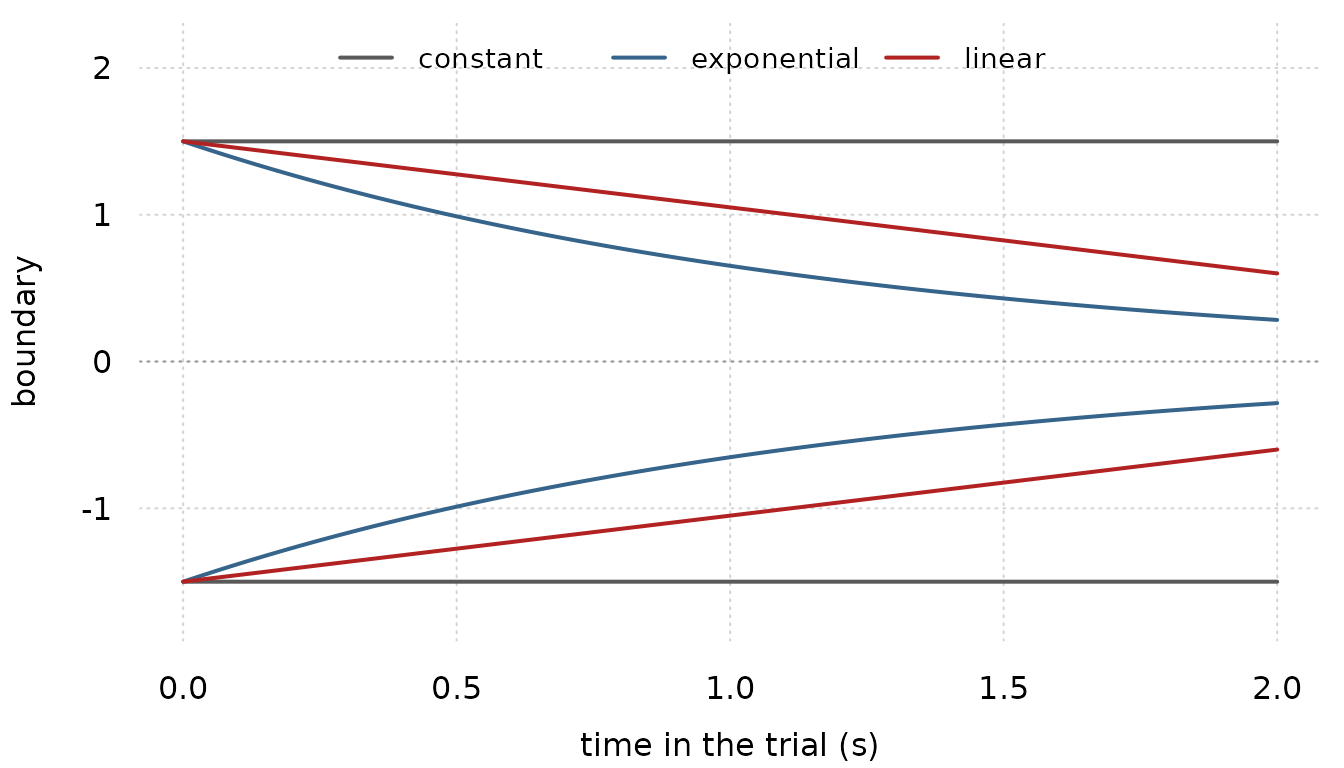

All three open at the same width. By the end of the trial the exponential pair has closed to about a fifth of it, so a slow decision needs a fifth of the evidence a fast one did, and what the accumulator runs between is a moving corridor rather than a fixed one.

Two responses is the whole of it. One accumulator in one dimension between two absorbing boundaries can end a trial at the upper wall or the lower wall and nowhere else, so multi-alternative choice is a different architecture rather than another parameter, and a third level in the decision indicator is refused rather than folded into one of the two.

An experiment

The design is the one the paper fits: a motion discrimination task at several coherences, where the drift grows with coherence and the boundaries collapse as the trial runs on.

gddm_simulate() draws from the model’s own density rather than from a forward simulation of the diffusion, whose first passages arrive late by however much the step misses excursions between monitoring times.

coh <- c(0, 0.128, 0.512)
ctl <- gddm_control(t_max = 2, dt = 0.02, ny = 101)
dat <- do.call(rbind, lapply(coh, function(cc) {
  gddm_simulate(300, mu = 6, alpha = 0.8, leak = 1, bs = 3, tau = 1.2,
                ndt = 0.25, coh = cc,
                drift = list(gddm_drift_coherence(cmax = 0.512),
                             gddm_drift_leak()),
                bound = gddm_bound_exponential(), control = ctl)
}))
dat$coh <- rep(coh, each = 300)
str(dat)
#> 'data.frame':    900 obs. of  4 variables:
#>  $ rt   : num  1.281 1.045 1.486 0.566 0.944 ...
#>  $ upper: int  0 0 1 0 0 0 1 1 1 1 ...
#>  $ cond : int  1 1 1 1 1 1 1 1 1 1 ...
#>  $ coh  : num  0 0 0 0 0 0 0 0 0 0 ...

Accuracy rises with coherence, and responses get faster:

data.frame(coh = coh,
           accuracy = round(tapply(dat$upper, dat$coh, mean), 3),
           mean_rt = round(tapply(dat$rt, dat$coh, mean), 3))
#>         coh accuracy mean_rt
#> 0     0.000     0.50   1.101
#> 0.128 0.128     0.98   0.807
#> 0.512 0.512     1.00   0.482

What the data must carry

Two things beyond the response time, and both are data.

Which boundary a trial ended at reaches the family through dec(), as it does for wiener(), or through vint(), which is the general-purpose route and the one used below. The condition a trial belongs to reaches it through vint(), and that one is particular to this family: one solve of the Fokker-Planck equation serves every trial that shares a parameter vector, and the family finds those trials through an index it is given rather than by comparing parameter values, which it cannot do on a tape.

vint() numbers its values positionally, so the two spellings put the condition in different places, and the family reads whichever it is:

rt | dec(response) + vint(cond)   # boundary in dec(), condition first
rt | vint(upper, cond)            # boundary first, condition second

gddm_conditions() builds the index. Name every variable that appears on the right-hand side of any formula in the model, and every covariate a drift term reads.

dat$cond <- gddm_conditions(dat, coh)
table(dat$cond)
#> 
#>   1   2   3 
#> 300 300 300

Naming more variables than you need is safe and only costs solves. Naming fewer is wrong, and wrong in a way nothing downstream can detect: the family checks that the covariates a drift reads are constant within a condition, but it cannot check the rest.

Fitting

fit <- frm(bf(rt | vint(upper, cond) + vreal(coh) ~ 1, bias = 0.5),
           family = gddm(drift = list(gddm_drift_coherence(cmax = 0.512),
                                      gddm_drift_leak()),
                         bound = gddm_bound_exponential(),
                         control = ctl),
           data = dat)
summary(fit)
#>  Family: gddm 
#>  Links: mu = identity; alpha = log; leak = identity; bs = log; tau = log;
#>         bias = logit; ndt = scaled_logit(0, 0.3267)
#> 
#> Formula: rt | vint(upper, cond) + vreal(coh) ~ 1 
#>    Data: dat (Number of observations: 900) 
#>  Method: ML   logLik: 46.4345   AIC: -80.869   BIC: -52.0547 
#> 
#> Regression Coefficients:
#>           Estimate Est.Error l-95% CI u-95% CI z value Pr(>|z|)
#> Intercept     5.68      0.23     5.22     6.14   24.21   <2e-16
#> 
#> Further Distributional Parameters:
#>       Estimate Est.Error l-95% CI u-95% CI
#> alpha     0.79      0.04     0.72     0.86
#> leak      0.73      0.65    -0.54     2.00
#> bs        3.07      0.45     2.31     4.08
#> tau       1.25      0.12     1.03     1.51
#> ndt       0.24      0.02     0.19     0.28
#> 
#> Fixed dpar: bias = 0.5

The estimates come back on the link scale, so put them back:

e <- unlist(fixef_by_dpar(fit))
data.frame(
  truth = c(mu = 6, alpha = 0.8, leak = 1, bs = 3, tau = 1.2, ndt = 0.25),
  estimate = round(c(
    mu = unname(e[["mu.(Intercept)"]]),
    alpha = exp(unname(e[["alpha.(Intercept)"]])),
    leak = unname(e[["leak.(Intercept)"]]),
    bs = exp(unname(e[["bs.(Intercept)"]])),
    tau = exp(unname(e[["tau.(Intercept)"]])),
    ndt = min(dat$rt) / (1 + exp(-unname(e[["ndt.(Intercept)"]])))), 3))
#>       truth estimate
#> mu     6.00    5.682
#> alpha  0.80    0.786
#> leak   1.00    0.731
#> bs     3.00    3.068
#> tau    1.20    1.247
#> ndt    0.25    0.241

bs is the separation between the boundaries, not the distance from the start to one of them, so it means what it means in wiener() and the two families’ estimates are directly comparable.

leak is positive for leaky integration and negative for unstable integration. It is the paper’s l, which is the negative of PyDDM’s leak.

The table of estimates is one reading of the fit. The other is the fitted distribution against the data it was fitted to, as defective cumulative distributions: one curve per wall, each leveling off at the proportion of trials that ended there.

# The solved density is not part of this package's API. These two are
# the internals its own solver tests read, and a picture of the fit
# needs the density on a grid, which nothing exported returns.
gd_solve <- frmtmb.eam:::gd_solve
gd_shift <- frmtmb.eam:::gd_shift
comp <- gddm(drift = list(gddm_drift_coherence(cmax = 0.512),
                          gddm_drift_leak()),
             bound = gddm_bound_exponential())[["gddm"]]$comp
est <- list(mu = unname(e[["mu.(Intercept)"]]),
            alpha = exp(unname(e[["alpha.(Intercept)"]])),
            leak = unname(e[["leak.(Intercept)"]]),
            bs = exp(unname(e[["bs.(Intercept)"]])),
            tau = exp(unname(e[["tau.(Intercept)"]])), bias = 0.5,
            ndt = min(dat$rt) / (1 + exp(-unname(e[["ndt.(Intercept)"]]))))

# one solve per condition, shifted by the non-decision time and
# renormalized exactly as the likelihood does it
gd_curve <- function(cov, dt = ctl$dt) {
  g <- list(dt = dt, ny = ctl$ny, t_max = ctl$t_max,
            nt = as.integer(round(ctl$t_max / dt)), tridiagonal = "recorded",
            wmax = as.integer(ceiling(est$ndt / dt)) + 2L)
  s <- gd_solve(est, cov, comp, g)
  u <- gd_shift(s$up, est$ndt, dt, g$wmax)
  l <- gd_shift(s$lo, est$ndt, dt, g$wmax)
  m <- (sum(u) + sum(l)) * dt
  data.frame(t = seq(0, ctl$t_max, by = dt), dt = dt,
             up = as.numeric(u) / m, lo = as.numeric(l) / m)
}
cv <- lapply(coh, gd_curve)
op <- par(mfrow = c(1, 3))
for (i in seq_along(coh)) {
  d <- dat[dat$coh == coh[i], ]
  g <- cv[[i]]
  # the panel is named with the variable rather than the word: the
  # theme's title is too large for a third of the width to hold
  # "coherence 0.512" without running off the last panel
  tinyplot::tinyplot(x = g$t, y = cumsum(g$up) * g$dt, type = "n",
                     theme = "clean2", xlim = c(0.2, 1.6), ylim = c(0, 1),
                     main = paste("coh", coh[i]),
                     xlab = "response time (s)",
                     ylab = "cumulative proportion")
  for (w in c(1, 0)) {
    cl <- if (w == 1) "steelblue4" else "firebrick"
    rt <- sort(d$rt[d$upper == w])
    lines(c(0.2, rt), c(0, seq_along(rt)) / nrow(d), type = "s", lty = 3,
          col = cl, lwd = 1.6)
    lines(g$t, cumsum(if (w == 1) g$up else g$lo) * g$dt, col = cl, lwd = 2)
  }
  if (i == 1) {
    legend("topleft", c("upper wall", "lower wall", "observed", "fitted"),
           col = c("steelblue4", "firebrick", "gray40", "gray40"),
           lty = c(1, 1, 3, 1), lwd = 2, bty = "n", cex = 0.95)
  }
}

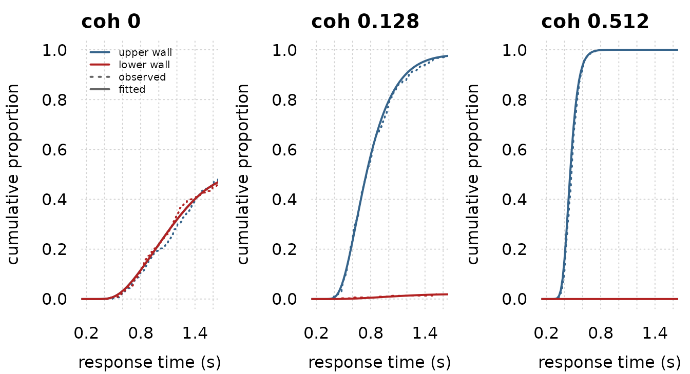
par(op)

The height a curve settles at is the choice proportion and its rise is the response times. The lower wall’s plateau falls from about a half at zero coherence to near zero at 0.512, and every fitted curve lies on its own observed steps.

The numerical scheme, and why it is this one

There is no density to evaluate, so every likelihood evaluation solves the Fokker-Planck equation forward in time and reads the probability flux through each boundary. Three things about how.

The boundaries are pinned, not chased. Substituting y = x / B(t) puts the walls at plus and minus one for all t. The spatial grid is then fixed while the boundary collapses, and no grid index depends on a parameter. This is what makes the model differentiable at all: the usual treatment sandwiches a moving bound between two integer grid indices, so the objective depends on where the bound falls between nodes, which is why the reference implementation fits by differential evolution and takes no derivatives.

The scheme is Crank-Nicolson. Once the walls are stationary it is available, and it is second order in the step and unconditionally stable. It is not available to a solver that chases the bound in the original coordinate: the discretized operator is stiff and its eigenvalues grow as the boundary collapses, so an explicit method would need a step orders of magnitude smaller.

The defective density is renormalized. The discretized solve loses a little probability mass, and how much it loses depends on the parameters, because a configuration that absorbs faster loses less. A likelihood that does not divide the loss out therefore pays a hidden bonus for absorbing quickly, and the bonus lands squarely on the leak and the boundary height. This is not a small effect: turning it off moves the leak by more than a factor of two on data simulated from the model itself. gddm_control(renormalize = FALSE) exists so the size of that bias can be measured, not because it is ever the better model.

Renormalizing also makes the density explicitly conditional on a response inside the modeled window, which is why t_max has to contain every response time and is worth setting to the experiment’s deadline when there is one.

How accurate, and how expensive

With a constant drift and boundaries that do not move, the generalized model is the Wiener model, so the solver can be checked against the closed form. At the shipped grid, over decision times from 0.2 s on and across a range of drifts, separations and starting points, the two agree to better than 0.01 in the log density. A coarser grid is worse and a finer one is better; the package’s own test suite pins all three.

ddm_lpdf_both <- frmtmb.eam:::ddm_lpdf_both
wcomp <- gddm()[["gddm"]]$comp
wp <- list(mu = 2, bs = 2, bias = 0.5, ndt = 0)
# no shift and no renormalization: the raw flux is what the closed form
# is a statement about, and it is what the solver tests compare
gd_raw <- function(dt, ny) {
  g <- list(dt = dt, ny = as.integer(ny), t_max = 2,
            nt = as.integer(round(2 / dt)), tridiagonal = "recorded")
  s <- gd_solve(wp, 0, wcomp, g)
  k <- 2:(round(1.5 / dt) + 1)
  tt <- seq(0, 2, by = dt)[k]
  data.frame(t = tt, up = pmax(as.numeric(s$up)[k], 1e-300),
             lo = pmax(as.numeric(s$lo)[k], 1e-300),
             eup = exp(ddm_lpdf_both(tt, 2, 2, 0.5, 1)),
             elo = exp(ddm_lpdf_both(tt, 2, 2, 0.5, 0)))
}
fine <- gd_raw(0.01, 201L)
crs <- gd_raw(0.02, 101L)
gd_err <- function(d) pmax(abs(log(d$up) - log(pmax(d$eup, 1e-300))),
                           abs(log(d$lo) - log(pmax(d$elo, 1e-300))))
sname <- c("closed form, upper", "closed form, lower", "solver, upper",
           "solver, lower")
scol <- c("gray70", "gray70", "steelblue4", "firebrick")
dens <- data.frame(t = rep(fine$t, 4),
                   d = c(fine$eup, fine$elo, fine$up, fine$lo),
                   s = factor(rep(sname, each = nrow(fine)), levels = sname))
err <- data.frame(t = c(fine$t, crs$t), e = c(gd_err(fine), gd_err(crs)),
                  g = factor(rep(c("dt 0.01, ny 201", "dt 0.02, ny 101"),
                                 c(nrow(fine), nrow(crs)))))
op <- par(mfrow = c(1, 2))
tinyplot::tinyplot(d ~ t | s, data = dens, type = "l", log = "xy",
                   theme = "clean2", col = scol, lwd = c(4, 4, 1.6, 1.6),
                   lty = c(1, 3, 1, 1), legend = FALSE, ylim = c(1e-12, 5),
                   main = "density, both walls",
                   xlab = "decision time (s)", ylab = "density")
legend("bottomright", sname, col = scol, lwd = c(4, 4, 1.6, 1.6),
       lty = c(1, 3, 1, 1), bty = "n", cex = 0.7)
tinyplot::tinyplot(e ~ t | g, data = err, type = "l", log = "xy",
                   theme = "clean2", col = c("steelblue4", "darkorange3"),
                   lwd = 2, legend = FALSE, main = "log-density error",
                   xlab = "decision time (s)", ylab = "absolute error")
abline(v = 0.2, lty = 2, col = "gray40")
abline(h = 0.01, lty = 2, col = "gray40")
legend("topright", levels(err$g), col = c("steelblue4", "darkorange3"),
       lwd = 2, lty = 1, bty = "n", cex = 0.7)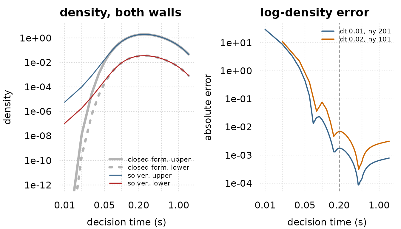

par(op)

Drawn at one drift and one separation, the solved density and the closed form are the same curve on both walls above about a twentieth of a second. Read as an error rather than as two curves, that same comparison is where the grid shows: past 0.2 s the coarser grid is about four times worse than the shipped one, and both stay well inside 0.01.

Two honest limits. The density at very short decision times, a few steps above zero, is much larger than the truth: an implicit scheme spreads a little mass everywhere immediately, where the true first-passage density is exponentially small. On a logarithmic density axis the closed form falls away to nothing at the left edge while the solver’s own curves carry on almost straight. It is small in absolute terms, and adding a lapse component floors it, but a fit should not be asked to read it. And refining ny alone helps only because the starting mass is deliberately spread over two grid cells rather than one; a sharper start would ring, because Crank-Nicolson does not damp the highest frequencies a grid carries.

The cost scales with the number of conditions, not the number of trials, because one solve serves a whole condition. It also scales with t_max / dt. Both the tape build and the evaluation grow with them, and gddm_control(tridiagonal =) trades one against the other: the default records the solve into the tape, which is slow to build and fast to run, while "atomic" collapses it into a single node with a hand-written derivative, which is quick to build and slower to run. The default suits a fit, which evaluates the objective many times.

Checked against PyDDM

The closed form above is only a check on the part of this family that is not generalized. With a constant drift and fixed bounds the model is the Wiener model and the solver can be held to the Navarro-Fuss density; nothing in that comparison reaches the leak, the collapsing bounds, the coherence nonlinearity, the start-point variability or the lapse, which are the reasons to use this family at all. Gradient tests show the derivative matches the value it is the derivative of, which is equally true of a wrong density, and parameter recovery is circular here on purpose, because gddm_simulate() draws from the solver’s own density.

So the generalized components are checked against PyDDM, the reference implementation of the model in Shinn et al. (2020). PyDDM discretizes the same equation in an unrelated way: a fixed grid in the original coordinate with the moving boundary sandwiched between the two nodes around it, where this package changes variable so that the boundary is pinned and the grid never moves. Ten cases are frozen into a fixture, and tests/testthat/test-gddm-reference.R reads it. No Python runs when the tests run; the fixture is regenerated by hand with dev/gddm-pyddm-reference.py in the source repository, and the test asserts its metadata so that a regenerated fixture cannot quietly redefine what is correct.

What the reference covers. A constant drift with fixed bounds, as calibration; a biased point start with a long non-decision time; leaky and unstable integration, one for each sign of leak; an exponentially collapsing bound; a linearly collapsing bound; the coherence nonlinearity at two coherences, which is the pair that pins alpha; uniform start-point variability; and a uniform lapse. For each of these, three things: the defective density at both boundaries on a common time grid, the two boundary masses, and the log-likelihood of a small fixed dataset whose response times fall between grid nodes, so that the likelihood’s own interpolation is exercised. At the shipped grid the two agree to between 7e-4 and 1.6e-3 in the log density on every case but one, which is an order of magnitude better than the 0.01 claimed above, and the test also requires the disagreement to shrink as dt and ny are refined, so the reference is what the solver converges to rather than merely something it lands near.

What the reference does not cover. The leading edge: within a few steps of zero both solvers spread a little mass where the true first-passage density is exponentially small, for the same structural reason, so the comparison starts at a decision time of 0.2 s and says nothing below it. Anything outside those ten cases, in particular a component you write yourself. Fitting: this compares densities, not estimates. And the two packages differ in two conventions that are translated rather than tested: this family renormalizes each condition’s pair of densities so that its likelihood is conditional on a response inside the window, while PyDDM keeps the undecided mass; and this family spreads a lapse over t_max where PyDDM spreads it over one time step more.

Where they disagree. On the exponentially collapsing bound the two sit 2.8e-3 apart in the log density, and refining this package’s grid alone does not close it. That is the reference’s error, not this package’s, and the way to see it is to refine the REFERENCE. PyDDM has no Crank-Nicolson path for a boundary that moves, so it solves that case with backward Euler on a grid-snapped bound, first order in both steps, and its own recorded convergence residual is 2.6e-3. Solved one level finer and extrapolated to zero step, PyDDM moves toward this package: measured against that limit rather than against the frozen fixture, gddm() is 8.1e-4 out at the shipped grid, then 2.8e-4, then 1.7e-4 as its own grid is refined. 8.1e-4 is inside the band the other nine cases occupy, so there is no floor here and nothing about this case that gddm() gets wrong.

The same is true of the start-variability case, which looks as though it settles at 2.6e-4. ICRange lays the uniform start on whole grid cells, so PyDDM’s box is about one cell too wide, an error first order in its spatial step. Against PyDDM’s extrapolated limit gddm() runs 7.2e-4, 2.1e-4, 6.5e-5 over the same three grids, which is the ordinary second-order sequence. In both cases the mechanism is a first-order error in the reference, and in both gddm() is the more accurate of the two: holding the walls still, and spreading the start with an integrated cubic B-spline instead of snapping it to cells, is what buys that.

A third opinion. Both packages march a partial differential equation on a grid, so agreeing with each other does not rule out an error they make in the same direction. The test also simulates the stochastic differential equation directly by Euler-Maruyama on the collapsing-bound case, where a shared error would be least surprising. A simulated first passage is late, because absorption is only noticed at a monitoring time, so two monitoring gaps driven by the same Brownian path are extrapolated to zero gap. It agrees with both packages to one or two standard errors, and it resolves a shared bias down to roughly two parts in a thousand. It is the size of those gaps that carries the conclusion and not which side of the reference a run falls on: the two quantities compared are anti-correlated by construction, so landing on opposite sides is the null expectation rather than evidence, and the observed sides change with the seed.

When a row falls off the grid

The density is floored before it is logged. Where the solved density at a trial’s own response time underflows, the log density is a large finite negative number rather than NaN. That matters twice: NaN is not a value a line search can use, and inside mixture() one NaN takes every other component with it through the log-sum-exp. The floored row is flat, so its gradient is exactly zero, which is what makes it harmless rather than merely quiet.

Being quiet is the cost, so the count is available to read:

gddm_floored(fit)
#> [1] 0
#> attr(,"rows")
#> integer(0)
#> attr(,"n_obs")
#> [1] 900

Zero means the grid represented every observation. A few rows means a few trials sit within a few time steps of the fitted non-decision time, where a fixed grid cannot resolve a density that is climbing through orders of magnitude, and those rows contributed a constant rather than information. Many rows means the fit is not to be trusted: shrink dt, or give the model a lapse component, which floors the density in the model rather than in the arithmetic.

The floor is reached where the solved density underflows, and that is the leading edge, just past the fitted non-decision time. The step decides what happens there, on the model fitted above.

gv <- do.call(rbind, lapply(c(0.04, 0.02, 0.01),
                            function(d) gd_curve(0.512, dt = d)))
gv <- gv[gv$t > 0.2 & gv$t < 0.62, ]
gv$step <- factor(paste("dt", gv$dt))
gcol <- c("steelblue4", "darkorange3", "firebrick")
tinyplot::tinyplot(pmax(up, 1e-14) ~ t | step, data = gv, type = "l",
                   log = "y", theme = "clean2", lwd = 2, legend = FALSE,
                   col = gcol, ylim = c(1e-13, 20),
                   xlab = "response time (s)", ylab = "density",
                   main = "upper wall at coherence 0.512")
abline(v = est$ndt, lty = 2, col = "gray40")
legend("bottomright", levels(gv$step), col = gcol, lwd = 2, lty = 1,
       bty = "n", cex = 0.85)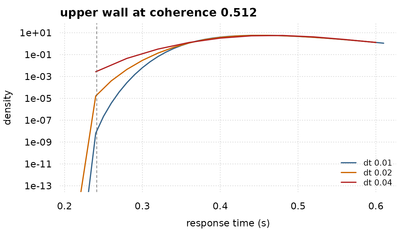

The three grids agree from about 0.4 s on. Below that they do not: at 0.28 s the coarsest is two orders of magnitude above the finest. It is those few nodes at the leading edge, not the bulk, that a smaller dt buys.

When not to use this

Use wiener() whenever it applies. That is whenever the drift is constant in the state and in time and the boundaries do not move: there the first-passage density is a known pair of series and costs arithmetic, while here every evaluation solves a partial differential equation once per condition. The difference is orders of magnitude.

What gddm() buys is the class of models the closed form cannot express at all. If the scientific question is whether the boundaries collapse, or whether integration is leaky, there is no analytic alternative to compare against.

Writing your own component

The catalogue is meant to be extended. A drift term is the value of gddm_drift_term(), a boundary is gddm_bound_term() and a starting distribution is gddm_start_term(). Each carries its own free parameters, each of which then takes a formula like any other.

A boundary that decays toward a floor rather than toward zero, say:

bound_floor <- function() {
  gddm_bound_term(
    "floored",
    dpars = list(
      bs = list(link = "log", init = function(y, aterms) 1.5),
      tau = list(link = "log", init = function(y, aterms) max(y)),
      floor = list(link = "logit", init = function(y, aterms) 0.3)),
    fn = function(t, p, ctl) {
      f <- p$floor + (1 - p$floor) * exp(-t / p$tau)
      list(B = 0.5 * p$bs * f,
           dlogB = -((1 - p$floor) / p$tau) * exp(-t / p$tau) / f)
    })
}
gddm(bound = bound_floor())[["dpars"]]
#> [1] "mu"    "bs"    "tau"   "floor" "bias"  "ndt"

Two rules. Nothing in a component may compare a parameter against anything, because a tape records no comparisons. And a boundary returns its logarithmic derivative alongside its value, because the change of variable that pins the walls needs it and differencing the boundary would cost the scheme its accuracy.

References

Broadie, M., Glasserman, P. and Kou, S. (1997). A continuity correction for discrete barrier options. Mathematical Finance, 7(4), 325-349. The result behind the Euler-Maruyama extrapolation: a first passage noticed only at a monitoring time is late by an amount of the order of the square root of the monitoring gap, not of the gap.

Shinn, M., Lam, N. H. and Murray, J. D. (2020). A flexible framework for simulating and fitting generalized drift-diffusion models. eLife, 9, e56938.