Differential equation models • frmtmb.ode

Some models say what the rate of change of a quantity is, not what the quantity is. A drug moves from a depot into the blood and is cleared from it; a population grows and is eaten. frm_ode() puts such a system inside a nonlinear formula, so the constants of the system are ordinary nonlinear parameters with fixed effects, random effects and covariates, and the model is fitted by maximum likelihood like any other frm() model.

Setup

frm_ode() is in frmtmb.ode, a package of its own that adds the solver to frmtmb’s formula grammar. Both live in the same repository:

remotes::install_github("aforren1/frmtmb", subdir = "extensions/frmtmb.ode")

It needs the RTMBode package in turn, which supplies a differentiable interface to the deSolve integrators. RTMBode is not on CRAN:

install.packages("RTMBode", repos = c(
  "https://kaskr.r-universe.dev",
  "https://cloud.r-project.org"))

Everything below is skipped if RTMBode is not installed.

A population pharmacokinetic model

The standard one-compartment model with first-order oral absorption has two states: the amount A still in the depot, and the concentration C in the central compartment.

$\frac{dA}{dt} = -k_a A, \qquad \frac{dC}{dt} = \frac{k_a A}{V} - k_e C$

A single dose D enters the depot at time zero, so $A(0) = D$ and $C(0) = 0$ . Three constants describe a subject: the absorption rate $k_a$ , the elimination rate $k_e$ , and the apparent volume of distribution $V$ . All three must be positive, so they are estimated on the log scale.

The system itself is a plain R function in the deSolve convention: it takes the time, the state vector and the parameter vector, and it returns the derivatives in a list. Index y and p by position. RTMB’s tape-safe c() and [<- replacements are in scope automatically, so the function needs no RTMB::ADoverload() boilerplate; only a helper function it calls, defined elsewhere, still needs its own bindings.

pk_dyn <- function(t, y, p) {
  list(c(-p[1] * y[1],
         p[1] * y[1] / p[3] - p[2] * y[2]))
}

datasets::Theoph is the classic example: 12 subjects, one oral dose of theophylline each, 11 serum concentrations over 25 hours.

d <- datasets::Theoph
d$Subject <- factor(as.character(d$Subject))
head(d, 3)
#> Grouped Data: conc ~ Time | Subject
#>   Subject   Wt Dose Time conc
#> 1       1 79.6 4.02 0.00 0.74
#> 2       1 79.6 4.02 0.25 2.84
#> 3       1 79.6 4.02 0.57 6.57

A pharmacokinetic dataset usually arrives in the layout NONMEM defined: one table, one row per record, with an evid column that says whether the row is an observation (0) or a dose (1), and amt and cmt on the dose rows. Here is Theoph in that layout, one dose record per subject into compartment 1, the depot. Each time-0 sample is listed before its dose, which in NONMEM order makes it the pre-dose sample:

dose_rec <- d[!duplicated(d$Subject), c("Subject", "Time", "Dose")]
dose_rec$Time <- 0
rec <- rbind(
  data.frame(Subject = d$Subject, Time = d$Time, evid = 0, amt = 0,
             cmt = 2, conc = d$conc),
  data.frame(Subject = dose_rec$Subject, Time = 0, evid = 1,
             amt = dose_rec$Dose, cmt = 1, conc = NA))
rec <- rec[order(rec$Subject, rec$Time, rec$evid), ]
head(rec, 3)
#>     Subject Time evid  amt cmt conc
#> 1         1 0.00    0 0.00   2 0.74
#> 133       1 0.00    1 4.02   1   NA
#> 2         1 0.25    0 0.00   2 2.84

frm_ode_records() splits such a table into the two things frm_ode() reads: the observations, which are the rows of the data, and the doses, which become the events table. It only reshapes: a dose means what its record says, and a record it cannot read that way is refused by name.

theo <- frm_ode_records(rec, id = "Subject", time = "Time")
doses <- theo$events
head(doses, 3)
#>   group time state value method duration ii addl    ss
#> 1     1    0     1  4.02    add        0  0    0 FALSE
#> 2    10    0     1  5.50    add        0  0    0 FALSE
#> 3    11    0     1  4.92    add        0  0    0 FALSE

The model is one bf(nl = TRUE) formula. The body says how a concentration is produced; the three nonlinear parameter formulas say how each constant varies between subjects. Both compartments start empty, and the dose arrives as an event. The solver tolerances are tightened from the default 1e-8 to 1e-10: at the default, this fit stops with nlminb reporting false convergence and a gradient of 1.7e-03, at a log likelihood 9e-08 from the tight fit. That is the integrator’s error showing through as noise in the objective.

form <- bf(
  conc ~ frm_ode(pk_dyn,
                 init   = list(0, 0),
                 times  = Time,
                 parms  = list(exp(lka), exp(lke), exp(lV)),
                 group  = Subject,
                 states = c("depot", "central"),
                 output = "central",
                 events = doses,
                 atol   = 1e-10,
                 rtol   = 1e-10),
  lka ~ 1 + (1 | Subject),
  lke ~ 1 + (1 | Subject),
  lV  ~ 1,
  nl = TRUE
)

fit <- frm(form + gaussian(), data = theo$data, se = TRUE,
           start = list(beta = c(0.5, log(0.08), log(0.5))))
summary(fit)
#>  Family: gaussian 
#>  Links: mu = identity; sigma = log
#> 
#> Formula: conc ~ frm_ode(pk_dyn, init = list(0, 0), times = Time, parms = list(exp(lka), exp(lke), exp(lV)), group = Subject, states = c("depot", "central"), output = "central", events = doses, atol = 1e-10, rtol = 1e-10) 
#>    Data: theo$data (Number of observations: 132) 
#>  Method: ML   logLik: -191.192   AIC: 394.384   BIC: 411.68 
#> 
#> Multilevel Hyperparameters:
#> ~Subject (Number of levels: 12) 
#>                   Estimate Est.Error l-95% CI u-95% CI
#> sd(lka_Intercept)     0.69      0.16     0.43     1.09
#> sd(lke_Intercept)     0.36      0.08     0.23     0.56
#> 
#> Regression Coefficients:
#>               Estimate Est.Error l-95% CI u-95% CI z value Pr(>|z|)
#> lka_Intercept     0.38      0.21    -0.03     0.79    1.82    0.069
#> lke_Intercept    -2.37      0.12    -2.61    -2.14  -19.97   <2e-16
#> lV_Intercept     -0.82      0.03    -0.87    -0.77  -30.82   <2e-16
#> 
#> Further Distributional Parameters:
#>       Estimate Est.Error l-95% CI u-95% CI
#> sigma      0.8      0.05      0.7     0.91

The typical subject’s constants come back on the natural scale, and the derived quantities a pharmacokineticist reads off them follow:

ka <- exp(fixef_by_dpar(fit)$lka); ke <- exp(fixef_by_dpar(fit)$lke)
V <- exp(fixef_by_dpar(fit)$lV)
c(ka = ka, ke = ke, V = V,
  half_life = log(2) / ke,       # hours
  clearance = ke * V)            # L/h per kg of body weight
#>        ka.(Intercept)        ke.(Intercept)         V.(Intercept) 
#>            1.46004483            0.09321159            0.43992080 
#> half_life.(Intercept) clearance.(Intercept) 
#>            7.43627637            0.04100572

Everything downstream works as usual: frm_linpred() on new times, ranef() for the subject deviations, confint(), simulate(), REML = TRUE. The dosing table names every subject, and frm_ode() refuses an events$group that the new data do not have, so new data carry every subject:

nd <- expand.grid(Time = seq(0, 25, length.out = 5),
                  Subject = levels(d$Subject))
nd$conc <- frm_linpred(fit, newdata = nd)
nd[nd$Subject == "1", ]
#>    Time Subject     conc
#> 1  0.00       1 0.000000
#> 2  6.25       1 7.257109
#> 3 12.50       1 5.663743
#> 4 18.75       1 4.420213
#> 5 25.00       1 3.449711

The same call on a dense time grid draws the fitted curve for every subject over that subject’s own observations. Each curve carries that subject’s random effects, which is why they differ in both height and shape.

grid <- do.call(rbind, lapply(split(d, d$Subject), function(s) {
  data.frame(Subject = s$Subject[1],
             Time = seq(0, max(d$Time), length.out = 100),
             Dose = s$Dose[1])
}))
grid$conc <- frm_linpred(fit, newdata = grid)

tinyplot::tinyplot(conc ~ Time | Subject, data = d, pch = 16, cex = 0.7,
                   legend = FALSE, xlab = "Time (h)",
                   ylab = "Concentration (mg/L)",
                   main = "Theophylline, fitted per subject")
tinyplot::tinyplot_add(conc ~ Time | Subject, data = grid, type = "l")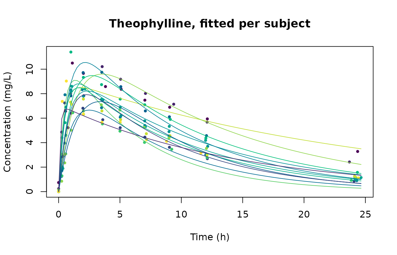

Theophylline concentration against time for twelve subjects, with the fitted curve of each subject drawn through its own points.

Each subject is observed once, so the curve and the points share a colour. The absorption peak moves between subjects because lka has a random effect.

How the arguments work

frm_ode() runs one solve per group, over that group’s own observation times, then puts the results back in the row order of the data.

Argument	What it is
first argument	The derivative function, `function(t, y, parms)`.
`init`	Initial states, one list element per state.
`times`	The observation time of every row.
`parms`	The constants of the system, one list element per constant, in the order the derivative function indexes them.
`group`	The unit that owns one system: a subject, a reactor, a batch.
`states`, `output`	State names, and which of them the body returns.
`t0`	The initial time. Defaults to 0.
`events`, `event_scale`	A dosing table, and an estimated multiplier on its amounts.
`tv`, `tv_break`	Constants that change with time, and where they change.
`n_ss`, `ss_tol`, `ss_extrapolate`	The length of a steady-state run-in, whether its tail is summed, and when to complain about it.
`method`, `atol`, `rtol`	Integrator and tolerances.

init and parms are given as lists of columns, not as one row of values per state. Each element is either one value per observation or a single value shared by every group. init = list(Dose, 0) is therefore “the depot starts at this row’s Dose, the central compartment starts at zero”. A bare vector such as c(100, 0) is refused, because it cannot be told apart from one column of two observations.

With no output the result is a matrix with one column per state, so frm_ode(...)[, 2] also works. Naming the states and selecting one by name is clearer and is what the example above does.

Repeated dosing

Theophylline is a single dose, so the dose could equally be written as the initial condition, init = list(Dose, 0), with no events; the two spellings give the same fit. A course of treatment cannot be written that way: the depot is refilled at each dose time, and the trajectory is the sum of what every dose so far has contributed. events is the table of those doses.

doses <- data.frame(time = c(12, 24, 36), state = "depot", value = 100)
doses
#>   time state value
#> 1   12 depot   100
#> 2   24 depot   100
#> 3   36 depot   100

One row per dose. time is when, state is which compartment (by name if states names them, otherwise by position), value is how much, and the default method = "add" puts the amount into the state. Give a row a positive duration and it becomes an infusion instead, delivering value at a constant rate over [time, time + duration]. A group column restricts a row to one subject; leave the column out and the schedule applies to every subject.

A regular course does not have to be written out. ii is the interdose interval and addl the number of doses that follow the row’s own, so these two tables are the same table:

data.frame(time = 0, state = "depot", value = 100, ii = 12, addl = 3)
#>   time state value ii addl
#> 1    0 depot   100 12    3
data.frame(time = c(0, 12, 24, 36), state = "depot", value = 100)
#>   time state value
#> 1    0 depot   100
#> 2   12 depot   100
#> 3   24 depot   100
#> 4   36 depot   100

The expansion happens before anything else looks at the table, so the two give bit-identical results.

In NONMEM terms an "add" row is a dosing record, value is amt, state is cmt, duration sets rate = amt / duration, and ii and addl are spelled the same way. There is no evid column, because observations and doses live in two separate tables here: the rows of data are the observations, the rows of events are the doses. frm_ode_records(), used on Theoph above, turns a NONMEM-shaped table into the two.

Solving directly, with the first dose as the initial condition and three more as events:

tt <- seq(0, 60, by = 0.25)
traj <- frm_ode(pk_dyn, init = list(100, 0), times = tt,
                parms = list(1, 0.2, 10),
                states = c("depot", "central"), output = "central",
                events = doses)
range(traj)
#> [1] 0.000000 7.522638

tinyplot::tinyplot(tt, traj, type = "l", lwd = 2,
                   xlab = "Time (h)", ylab = "Concentration (mg/L)",
                   main = "Four doses, twelve hours apart")
abline(v = c(0, doses$time), lty = 3, col = "grey40")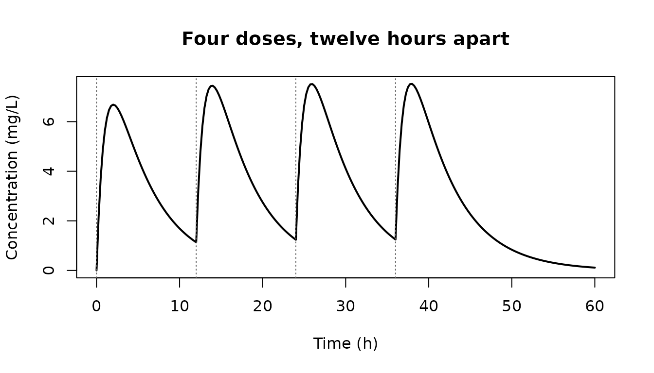

Concentration against time for four doses given twelve hours apart, rising to a plateau, with a vertical line at each dose time.

Each peak is higher than the last and the troughs level off, so the course approaches a steady state instead of repeating the first dose. That accumulation is why a dosing schedule cannot be faked with one larger dose.

Inside a formula

A nonlinear body looks up every bare name in data first, so a column called doses wins. There is no column of that name here, and a data.frame is not something a column could hold, so the table is read from the environment of the formula:

conc ~ frm_ode(pk_dyn, init = list(0, 0), times = time,
               parms = list(exp(lka), exp(lke), exp(lV)),
               group = id, states = c("depot", "central"),
               output = "central", events = doses)

Writing the table inline says the same thing, and a function of no arguments is the way to read the schedule at fit time:

conc ~ frm_ode(pk_dyn, ..., events = data.frame(
                 time = c(0, 12, 24), state = "depot", value = 100))

schedule <- function() read.csv("doses.csv")
conc ~ frm_ode(pk_dyn, ..., events = schedule)

A fit is otherwise unchanged. Here is a small simulated course of three doses twelve hours apart, with between-subject variability on lka and lke:

set.seed(4)
n_id <- 8
tt_obs <- c(0.5, 2, 6, 11.9, 14, 20, 23.9, 26, 32, 40)
dd <- data.frame(id = factor(rep(seq_len(n_id), each = length(tt_obs))),
                 time = rep(tt_obs, n_id))
ka_i <- exp(rnorm(n_id, 0, 0.3))[as.integer(dd$id)]
ke_i <- exp(rnorm(n_id, log(0.2), 0.25))[as.integer(dd$id)]
super <- function(t, ka, ke, V, amt, at) {
  u <- t - at[at <= t]
  sum(amt * ka / (V * (ka - ke)) * (exp(-ke * u) - exp(-ka * u)))
}
dd$conc <- vapply(seq_len(nrow(dd)), function(i)
  super(dd$time[i], ka_i[i], ke_i[i], 10, 100, c(0, 12, 24)), 0) +
  rnorm(nrow(dd), 0, 0.3)

dose_fit <- frm(
  bf(conc ~ frm_ode(pk_dyn, init = list(100, 0), times = time,
                    parms = list(exp(lka), exp(lke), exp(lV)),
                    group = id, states = c("depot", "central"),
                    output = "central",
                    events = data.frame(time = c(12, 24),
                                        state = "depot", value = 100)),
     lka ~ 1 + (1 | id), lke ~ 1 + (1 | id), lV ~ 1, nl = TRUE) +
    gaussian(),
  data = dd, start = list(beta = c(0, log(0.25), log(8))))
unlist(fixef_by_dpar(dose_fit))
#>   lka.(Intercept)   lke.(Intercept)    lV.(Intercept) sigma.(Intercept) 
#>        0.04225596       -1.44209990        2.28231919       -1.30575528

The truth is lka = 0, lke = -1.61 and lV = 2.30, with a residual standard deviation of 0.3, which is -1.20 on the log scale sigma is reported on.

show <- levels(dd$id)[1:4]
sub <- dd[dd$id %in% show, ]
sub$id <- droplevels(sub$id)
gr <- do.call(rbind, lapply(show, function(s)
  data.frame(id = factor(s, levels = levels(dd$id)),
             time = seq(0, 40, length.out = 200))))
gr$conc <- frm_linpred(dose_fit, newdata = gr)
gr$id <- droplevels(gr$id)

tinyplot::tinyplot(conc ~ time | id, data = sub, pch = 16,
                   xlab = "Time (h)", ylab = "Concentration (mg/L)",
                   main = "Three doses, four subjects")
tinyplot::tinyplot_add(conc ~ time | id, data = gr, type = "l")
abline(v = c(0, 12, 24), lty = 3, col = "grey40")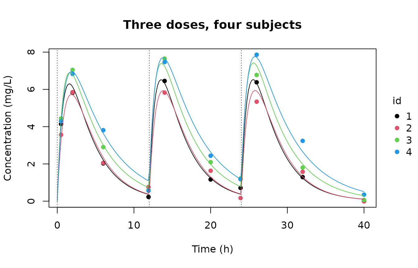

Observed concentrations and fitted curves for four subjects on a three dose course, with a vertical line at each dose time.

Doses that depend on a parameter

events$value is a numeric column, so it cannot hold something being estimated. event_scale is the way in: one value per observation, constant within group, multiplying every amount in that group. A bioavailability is then an ordinary nonlinear parameter, free to carry covariates and random effects:

bf(conc ~ frm_ode(pk_dyn, init = list(0, 0), times = time,
                  parms = list(exp(lka), exp(lke), exp(lV)),
                  group = id, states = c("depot", "central"),
                  output = "central",
                  events = data.frame(time = c(0, 12, 24),
                                      state = "depot", value = 100),
                  event_scale = 1 / (1 + exp(-logitF))),
   lka ~ 1 + (1 | id), lke ~ 1 + (1 | id), lV ~ 1, logitF ~ 1, nl = TRUE)

Because scaling is only meaningful for an amount, event_scale is refused on a table containing "replace" or "multiply" rows.

An observation at a dose time is the trough

An observation whose time equals a dose time reads the state before that dose, which is the pre-dose sample a study protocol asks for. That also covers an observation at t0 when a dose is given at t0: it reads init. If you want the post-dose value, ask for a time just after.

How the doses are applied

frm_ode() does not hand the table to deSolve’s own events argument. It splits the integration at the event times instead, and chains one solve per interval, carrying the state across the break itself.

That is a correctness requirement. RTMBode integrates an augmented system that carries the derivative of each state with respect to each parameter alongside the states. A deSolve event jumps the state and leaves those derivatives untouched, which is right for an addition and wrong for the other two methods: measured against finite differences, "replace" and "multiply" came out 42% and 59% off. Splitting the solve is exact for all three, and it is what makes event_scale possible at all.

The price is one solve per dosing interval per group. A twice-daily regimen over a fortnight is 28 solves per subject, not one.

Starting at steady state

A patient on maintenance therapy was not dosed for the first time this morning. ss = TRUE on a row says the cycle it describes has already been running long enough to settle, and the row’s ii says how often:

ss_ev <- data.frame(time = 0, state = "depot", value = 100,
                    ii = 12, ss = TRUE)
tt <- c(0, 1, 3, 6, 11.9)
frm_ode(pk_dyn, init = list(0, 0), times = tt, parms = list(1, 0.2, 10),
        states = c("depot", "central"), output = "central",
        events = ss_ev)
#> [1] 1.247033 6.656660 6.922232 4.109565 1.272218

The steady state is reached by simulation, not by a formula, so it works for any dynamics: every compartment is set to zero, which is how NONMEM and rxode2 read a steady-state record and why the row overrides init, and the cycle is then repeated n_ss times before the record’s time. The record’s own dose lands afterwards, so an observation at the record’s time is the steady-state trough.

A real steady state is “repeat until the state at the start of the cycle stops moving”, and that test branches on a value, which the tape cannot do: the number of solves has to be fixed before the tape is built. Stopping at n_ss cycles leaves the state short of the limit, and for linear kinetics the shortfall is the accumulation factor to the power n, exp(-n * lambda_z * ii), where lambda_z is the slowest disposition rate. It grows toward 1 as the terminal half-life grows against the dosing interval.

That tail is a geometric series whose ratio the run-in has already measured, though. ss_extrapolate = TRUE, the default, reads the ratio off the last cycle-start differences and adds the rest of the sum. It is arithmetic on tape variables, so unlike the convergence test it runs during a fit, and it costs no extra solve.

A one-compartment intravenous model shows the size of both, because there the exact steady-state trough is known. Set a long half-life against the interval so the tail is worth summing:

decay <- function(t, y, p) {
  list(c(-p[1] * y[1]))
}
k <- 0.01                          # a half-life of 5.8 dosing intervals
iv_ss <- data.frame(time = 0, value = 100, ii = 12, ss = TRUE)
tr <- 100 * exp(-k * 12) / (1 - exp(-k * 12))        # the exact trough

short <- function(n, ext) {
  g <- frm_ode(decay, init = list(0), times = 0, parms = list(k),
               events = iv_ss, n_ss = n, ss_tol = Inf,
               ss_extrapolate = ext, atol = 1e-10, rtol = 1e-10)
  abs(g - tr) / tr
}
rbind(truncated = vapply(c(4, 8, 20), short, 0, ext = FALSE),
      summed    = vapply(c(4, 8, 20), short, 0, ext = TRUE))
#>                   [,1]         [,2]         [,3]
#> truncated 6.187834e-01 3.828929e-01 9.071795e-02
#> summed    5.937775e-10 6.675075e-10 7.552169e-10

The truncated row is exp(-n * k * 12) exactly. The summed row is the integrator’s own tolerance, not the run-in’s, at every n_ss in it.

The correction is exact for linear kinetics only up to the second-slowest mode, so it is not a licence to stop thinking about n_ss. On a strongly nonlinear system it helps less, and on flip-flop absorption, where ka is near lambda_z, it can be worse than truncating: measured over 338 two-compartment oral cycle maps it loses on 8 of them, worst by a factor of 2.27. That is bounded and it is why the default stays TRUE. The smallest error truncation leaves on a losing case is 0.40 of the trajectory’s own scale, so the correction never loses where truncation was usable, and the warning below fires on every losing case in both arms. ?frm_ode has the mechanism.

Off the tape frm_ode() says how far the answer it returned still is from the limit, and warns when that is more than ss_tol; it also says so by name when a state is not contracting between cycles at all, which means no n_ss settles it. Read that number as a DETECTOR rather than a measurement: it comes from the same geometric model the correction does, so where the model is poor it is poor with it. During a fit the comparison cannot run at all, so read the warning from a frm_linpred() or a direct call. ss_extrapolate = FALSE restores the truncated run-in bit for bit.

Raising n_ss a long way has its own limit. The cycles are chained solves, so the integrator’s error accumulates over all of them: at the default tolerances and n_ss = 1000 it contributes about 2e-05, more than the run-in shortfall the extra cycles were bought to remove. Tighten atol and rtol alongside n_ss, or the extra cycles buy nothing.

The cost is n_ss extra solves per group either way, so a steady-state population fit is several times a plain one.

Resetting the system

method = "reset" sets every compartment to value. With value = 0 that is NONMEM’s and rxode2’s evid = 3: washout, a new period of a crossover, a dropped-and-restarted infusion.

frm_ode(pk_dyn, init = list(100, 0), times = c(1, 2, 3, 4),
        parms = list(1, 0.2, 10), output = 2L,
        events = data.frame(time = 2, value = 0, method = "reset"))
#> [1] 5.635641 6.687310 0.000000 0.000000

A reset and a dose at the same time is evid = 4, a reset dose. The reset is always applied first, so the order of the two rows in the table does not change the answer. A reset row names no compartment, so it needs no state even in a multi-state system, and event_scale leaves it alone: it sets a level, not an amount.

Covariates that change with time

init and parms are read off each group’s first row, so a covariate that changes within a subject cannot enter them. That is the right refusal for a constant, and the wrong answer for renal function, body weight over a long study, or an infusion of a second drug that changes the elimination of the first. tv is where those go.

tt <- c(1, 3, 6, 9, 12)
ke_t <- ifelse(tt < 6, 0.2, 0.4)         # elimination doubles at hour 6

pk_tv <- function(t, y, p) {
  # `tv` values follow `parms`, so ka is p[1], V is p[2], and the
  # time-varying ke is p[3]
  list(c(-p[1] * y[1],
         p[1] * y[1] / p[2] - p[3] * y[2]))
}

frm_ode(pk_tv, init = list(100, 0), times = tt, parms = list(1, 10),
        tv = list(ke_t), states = c("depot", "central"),
        output = "central")
#> [1] 5.6356414 6.2378071 3.7339432 1.1350284 0.3423811

The solve is split at each change point, exactly as it is split at a dose time, and each segment’s dynamics see that segment’s value. Nothing in the derivative function learns that anything changed: within a segment p[3] is an ordinary constant.

The step is last observation carried forward, which is the rule rxode2 uses for covariates. A row’s value is in force from that row’s time until the next change, and the first row’s value reaches back to t0. One consequence is worth stating, because it differs from a dose: the state is continuous across a change point, since a covariate moves the derivative and not the state. An observation exactly at a change point therefore reads what the pre-change dynamics produced, and the difference appears only afterwards. At a dose time the same observation reads the trough, because a dose does jump the state.

An estimated time-varying parameter

The values may be estimated. The change points may not: they decide where the solve is split, and that is settled before the tape is built. When a tv column carries estimated values there is nothing to compare, because RTMB refuses comparison on AD types, so tv_break names the data column whose changes mark them.

set.seed(77)
n_id <- 10
tt_obs <- c(0.5, 2, 4, 8, 11.9, 13, 16, 20)
dv <- data.frame(id = factor(rep(seq_len(n_id), each = length(tt_obs))),
                 time = rep(tt_obs, n_id))
dv$phase <- factor(ifelse(dv$time < 12, "early", "late"))
b_i <- rnorm(n_id, 0, 0.25)[as.integer(dv$id)]
k_e <- exp(log(0.15) + b_i)
k_l <- exp(log(0.15) + log(2) + b_i)
dv$conc <- ifelse(dv$time < 12,
                  100 * exp(-k_e * dv$time),
                  100 * exp(-k_e * 12) * exp(-k_l * (dv$time - 12))) +
  rnorm(nrow(dv), 0, 0.6)

tv_fit <- frm(
  bf(conc ~ frm_ode(decay, init = list(100), times = time,
                    tv = list(exp(lk)), tv_break = phase,
                    group = id, output = 1L),
     lk ~ 1 + phase + (1 | id), nl = TRUE) + gaussian(),
  data = dv, start = list(beta = c(log(0.2), 0)))
unlist(fixef_by_dpar(tv_fit))
#>    lk.(Intercept)      lk.phaselate sigma.(Intercept) 
#>       -1.78812648        0.75055986       -0.08544209

lk is a linear predictor that varies within a subject, which parms would refuse by name. In tv it is the whole point. The truth is lk = -1.90 early and a shift of log(2) = 0.69 late.

A tv column has no constant to be read off the first row, so parms may be left out entirely when every input varies with time.

Two measurements from one solve

A parent drug and its metabolite are measured on the same assay, one column of concentrations with a compartment label beside it. Two species of a predator-prey series stack the same way. Given one output value per row, frm_ode() solves the system once per group and each row reads the state its label names:

bf(y ~ frm_ode(pm_dyn, init = list(dose, 0, 0), times = time,
               parms = list(exp(lka), exp(lkm), exp(lke)),
               group = id, output = cmt),      # cmt is 2 or 3 per row
   lka ~ 1, lkm ~ 1, lke ~ 1, nl = TRUE)

Without this the model is written as two calls, one per state, selected by an indicator: the same likelihood at twice the solves. A per-row output is told apart from a selection of states by length: it needs one value per row, and more rows than the system has states.

A combined error model

Assay error in pharmacokinetics is rarely purely additive. The usual model is proportional plus additive,

$\mathrm{sd} = \sqrt{a^2 + (b\,\mu)^2},$

which nlf() writes directly, because an nlf() body may read another parameter’s per-row value. sigma is reported on the log scale, so the body is half the log of the variance:

bf(conc ~ frm_ode(pk_dyn, init = list(dose, 0), times = time,
                  parms = list(exp(lka), exp(lke), exp(lV)),
                  group = id, output = 2L),
   lka ~ 1 + (1 | id), lke ~ 1 + (1 | id), lV ~ 1, nl = TRUE) +
  nlf(sigma ~ 0.5 * log(exp(2 * ladd) + exp(2 * lprop) * mu^2)) +
  lf(ladd ~ 1, lprop ~ 1) + gaussian()

exp(ladd) is the additive component and exp(lprop) the proportional one, both on the log scale so both stay positive. This needs no new machinery: it is nlf() plus the ODE body, and the two components come back separately in fixef().

Three things that will bite

A covariate must not vary inside a group

frm_ode() reads each constant off the group’s first row, because one solve has one set of constants. A covariate that changes between an early and a late observation of the same subject therefore describes a model this helper cannot solve, and it is refused by name at frame assembly:

d$phase <- factor(ifelse(d$Time <= 2, "early", "late"))
frm(bf(conc ~ frm_ode(pk_dyn, init = list(Dose, 0), times = Time,
                      parms = list(exp(lka), exp(lke), exp(lV)),
                      group = Subject, output = 2L),
       lka ~ 1 + (1 | Subject),
       lke ~ 1 + phase + (1 | Subject),      # varies within Subject
       lV ~ 1, nl = TRUE) + gaussian(), data = d)
#> Error: Nonlinear parameter 'lke' is a dynamics input of frm_ode() but
#> is not constant within 'Subject': phaselate. ...

A covariate that is constant within a subject, such as weight or treatment arm, is the intended case: lV ~ 1 + Wt is fine. A covariate that really does change with time goes in tv instead, where the solve is split at each change; the refusal is for init and parms, which are read once.

Without the check the fit is quietly wrong rather than loud. The coefficient stays at its starting value, the log-likelihood does not move, and the only symptom is an indefinite Hessian.

Only adaptive integrators

A fixed-step integrator run at the default number of steps does not solve the system to the tolerance the likelihood is defined at, so it returns a different likelihood, not a noisier one: on the probe data rk4 reported -63.93 where lsoda, lsode, adams and ode45 all reported -60.46 to seven digits. frm_ode() refuses method = "rk4" and method = "euler". The default "lsoda" is both the fastest and the quietest of the adaptive methods.

Keep the system small

Each group’s system must be small. Above roughly eight states in one system, the second-order derivative path that the Laplace approximation needs starts returning NaN gradients, and with some integrators the process crashes. frm_ode() warns past that point. This is why groups are solved one at a time and never stacked into one large system, even though stacking would look like the obvious optimization.

Compartment models live far below the ceiling, so in practice this only means: do not try to fold the subjects into the state vector yourself.

Cost

The tape is built once, but every gradient evaluation replays one adjoint solve per group, so the cost is linear in the number of groups and does not shrink with tape reuse. For the two-state model above, eight timepoints per subject, a whole frm() call including sdreport():

subjects	rows	with `frm_ode()`	with the closed form
6	48	1.6 s	0.05 s
12	96	3.5 s	0.06 s
25	200	8.3 s	0.08 s
50	400	19.9 s	0.11 s

About 0.4 s per subject. A 200-subject population model is a couple of minutes, and an intensively dosed one is much worse than that, because the solve is split at every dose: 100 subjects sampled eight times, dosed twice daily for a week and started from a steady state, is 3717 seconds, and that is not the data being large. It is 33 numerical solves per subject for every evaluation of the likelihood.

If your system is LINEAR, do not pay any of that. See the next section.

The linear case has a closed form

A one-, two- or three-compartment model with first-order absorption and first-order elimination is linear, and a linear system does not need an integrator. frm_lincmt() writes the analytic solution: the amount in a compartment is the superposition of the impulse responses of the doses that came before the observation, and a steady-state record is the geometric series of that superposition rather than a run-in.

It takes the same events table, the same group, the same event_scale, and it sits in a bf(nl = TRUE) body the same way. What changes is that the system is named rather than written:

form <- bf(
  conc ~ frm_lincmt(parms = list(ka = exp(lka), ke = exp(lke),
                                 V = exp(lV)),
                    times = Time, group = Subject,
                    ncmt = 1, depot = TRUE,
                    init = list(depot = Dose)),
  lka ~ 1 + (1 | Subject),
  lke ~ 1 + (1 | Subject),
  lV  ~ 1,
  nl = TRUE
)

ncmt counts the disposition compartments and depot says whether an absorption compartment feeds them. parms is named because which parameters a shape needs depends on those two, and it reads either rate constants (ke, k12, k21, k13, k31, ka, V) or clearances (CL, V, Q2, V2, Q3, V3, ka).

The two agree, and the closed form is far cheaper. On the design that costs 3717 s above, frm_lincmt() at its default takes 55 s, and the same fit with the steady-state run-in written out at n_ss = 20 takes 119 s. Comparing each arm’s slowest measurement against the other’s fastest, that is at least 67 times faster at the default and at least 31 times at n_ss = 20; at a size where all three fits are cheap enough to repeat, and where the optimizer takes the same number of iterations in each, the factors are 95 and 47. The two return the same estimates to seven significant digits (ka 0.9841612 against 0.9841609). On 118 schedules spanning bolus and infusion, single and repeated dosing, steady state, one to three compartments with and without a depot, they differ by at most 2.6e-12 of the trajectory’s own scale, and tightening the solver drives that difference down rather than leaving it, so it is frm_ode()’s tolerance and not the closed form’s error.

Three practical differences are worth knowing.

n_ss defaults to Inf. frm_lincmt() sums the steady-state series in closed form, so there is nothing to truncate and nothing to be short of. Passing a whole number writes that many cycles out instead, which is what reproduces frm_ode(ss_extrapolate = FALSE) exactly. frm_ode()’s default sums the tail its run-in truncates rather than dropping it, so the two DEFAULTS agree: on the two-compartment schedule in this package’s tests, truncating at twenty cycles leaves the state 0.4 percent short of the limit (0.00396 of the trajectory’s own scale) and summing the tail leaves it at the integrator’s tolerance.

It needs no solver. Neither RTMBode nor deSolve is involved, so frmtmb.sample::frm_sample() works on a frm_lincmt() model where it refuses a frm_ode() one.

It refuses what superposition cannot carry, by name rather than quietly: method = "replace" and method = "multiply", a "reset" to a non-zero level, a dose into or an output from a peripheral compartment, an infusion into the depot (that is zero-order absorption), tv, and an infusion still running when the schedule restarts. Every one of those is a model frm_ode() fits.

What is out of scope

Time-varying input that is not a step function. A branch on time inside the derivative function does not work, and it is worth knowing why. RTMBode tapes that function once, so t is an automatic-differentiation value inside it. Writing if (t < t_end) rate else 0 raises

Error: Comparison is generally unsafe for AD types

which is the good outcome. An approxfun() forcing table is the bad one: it silently returns the value at the taping point, so the model you fit is not the model you wrote. Smooth arithmetic in t, such as p[2] * exp(-p[3] * t), is fine. A piecewise-constant input belongs in tv, or in events as an infusion, where it rides along as a parameter over each interval and is differentiated exactly. deSolve’s own forcings argument is not reachable through RTMBode. Linear interpolation between measured covariate values, which rxode2 offers, is not available either: the value inside a segment would have to depend on t.

Estimated event times. Lag times, estimated inter-dose intervals, estimated observation times and estimated tv change points are not supported. They decide where the solve is split, and that is settled before the tape is built.

frm_linpred(se.fit = TRUE) is not available for any nonlinear predictor, frm_ode() included. Ask for a nonlinear parameter instead, with frm_linpred(dpar = "lka").

Failed solves

Mid-optimization the optimizer probes extreme rate constants, and a solve can fail there. on_error and penalty say what to do about that, but they reach less far than they look like they do, and the difference is worth knowing before you rely on them.

While fitting, most failures cannot be caught. The body runs on the automatic-differentiation tape. There RTMBode::ode() returns an AD object and raises no R error when a trajectory goes bad, and RTMB refuses comparison on AD types, so nothing can test the result for NaN. A diverging region of the parameter space therefore reaches you as the optimizer’s own warning,

Warning: NA/NaN gradient evaluation

and on_error = "error" will not name the group. Two failures are still caught on the tape: an integrator that gives up and returns fewer time points than it was asked for, and an R error raised by your derivative function.

Everywhere else every check applies. frm_linpred(), simulate(), residuals(), a direct call to frm_ode(), and a fit whose init and parms contain no estimated parameter are ordinary numeric arithmetic. There a failed solve is detected, and by default its rows are filled with penalty.

A penalty is never written silently. frm_ode() warns and names the groups, and frm_ode_failures() reads the record back afterwards:

p <- frm_linpred(fit, newdata = nd)
#> Warning: frm_ode(): the solve failed for 1 of 3 groups (2). Their rows
#> hold penalty = 1e+06, not a solution. ...

frm_ode_failures()
#> $groups
#> [1] "2"

Those rows are missing values dressed as numbers. Treat them as missing.

To localize an NA/NaN gradient from a fit, call frm_ode() yourself at the suspect parameter values with on_error = "error". Numerically it will name the group that cannot be solved.

Solver warnings from deSolve (“corrector convergence failed repeatedly”, “exceeded maxsteps”) during a fit are normal noise from those probing steps. Judge the fit by diagnose() and the gradient at the optimum, not by whether the solver complained on the way.