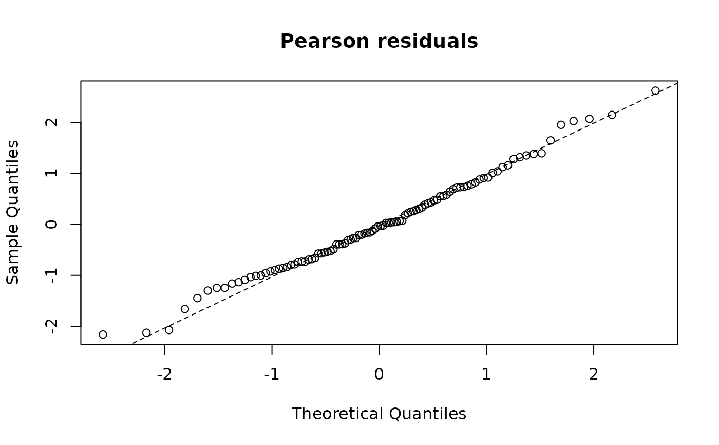
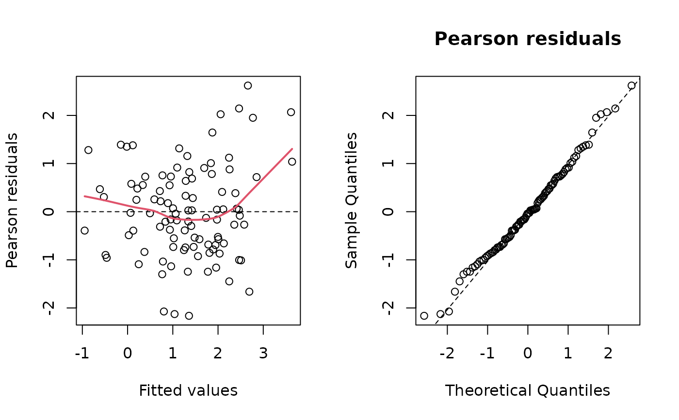
Panel 1: Pearson residuals against fitted values with a lowess
trend. Panel 2: normal QQ plot of the Pearson residuals. For
simulation-based residuals that are exact for discrete families, use
dharma_residuals() or residuals(type = "osa").
Usage
# S3 method for class 'frmtmb_fit'
plot(x, which = 1:2, ask = NULL, ...)
Arguments
- x
A
frmtmb_fit.- which
Subset of
1:2.- ask
Whether to prompt between plots; defaults to the usual interactive-device rule.
- ...
Refused: an argument the method does not have is an error naming it, rather than silently changing nothing. brms's
plot.brmsfit()arguments (N,nvariables,variable,regex,pars,fixed,combo,bins,theme,plot,newpage) are refused by name with the reason: they choose and lay out the per-parameter panels of posterior draws, and a maximum-likelihood fit has no draws and no such panels.
Details
On an ordinal fit fitted() is a matrix of category probabilities,
so panel 1 uses the expected category index sum_k k * P(y = k) -
the same scalar the Pearson residual is taken against - and labels
the axis accordingly.
brms's display
brms's plot() of a fit draws a histogram and a trace of the
posterior draws of each parameter, nvariables (or N) parameters
to a page, selected with variable and regex. A
maximum-likelihood fit has one estimate per parameter and no chains,
so this method draws the residual diagnostics a frequentist fit is
read with, and refuses brms's arguments by name. For brms's display,
sample and plot the draws:
plot(frmtmb.sample::frm_sample(fit), variable = "^b_", regex = TRUE).
For one parameter's likelihood, plot(profile(fit, parm)).
Examples
set.seed(1)
dd <- data.frame(x = rnorm(100), g = factor(rep(1:10, 10)))
dd$y <- rnorm(100, 1 + 0.5 * dd$x + rnorm(10, 0, 0.8)[dd$g], 1)
fit <- frm(bf(y ~ x + (1 | g)) + gaussian(), data = dd)
# both panels, side by side
op <- par(mfrow = c(1, 2))
plot(fit, ask = FALSE)
 par(op)
# just the QQ panel
plot(fit, which = 2)