Case studies: models from the showcase literature
Source:vignettes/case-studies.Rmd
case-studies.RmdEach section below takes a model that another package uses to show
what it can do, and fits it with frm(). Every section says
where the model comes from, gives the frmtmb call, reads the output, and
then checks the numbers against a package or a closed form that computes
the same thing a different way. The datasets are small so that this page
rebuilds in under a minute.
Most sections carry a figure. The figures use tinyplot, which is a suggested package, and they are skipped when it is not installed.
This is not the getting-started page. See
vignette("frmtmb") for the grammar and
vignette("brms-migration") for the brms feature map.
1. The animal model
The animal model is the flagship example of MCMCglmm (Hadfield 2010,
Journal of Statistical Software 33(2); see also Wilson et
al. 2010, Journal of Animal Ecology 79, “An ecologist’s guide
to the animal model”). It splits phenotypic variance into an additive
genetic part and a residual part. Each individual gets one random
effect, and those effects are correlated through the additive
relationship matrix A, which the pedigree determines. Two
individuals with relatedness 0.5, such as full sibs, share half of their
additive genetic deviation in expectation.
The relatedness matrix is not a column of data, so it
travels in data2, exactly as in brms.
gr(id, cov = A) attaches it to the grouping factor.
# a half-sib design: 12 sires, 2 dams each, 6 offspring per pair
nsire <- 12; ndam_per <- 2; noff <- 6
nfound <- nsire + nsire * ndam_per
n <- nfound + nsire * ndam_per * noff
ped <- data.frame(id = 1:n, sire = NA_integer_, dam = NA_integer_)
k <- nfound
for (s in 1:nsire) for (j in 1:ndam_per) {
  dam <- nsire + ndam_per * (s - 1) + j
  for (o in 1:noff) { k <- k + 1; ped$sire[k] <- s; ped$dam[k] <- dam }
}

# the tabular method builds A from a pedigree sorted parents-first
A <- diag(n)
for (i in seq_len(n)) {
  s <- ped$sire[i]; d <- ped$dam[i]
  if (!is.na(s)) {
    A[i, i] <- 1 + 0.5 * A[s, d]
    for (j in seq_len(i - 1)) A[i, j] <- A[j, i] <- 0.5 * (A[j, s] + A[j, d])
  }
}
dimnames(A) <- list(as.character(ped$id), as.character(ped$id))

set.seed(9)
dat <- data.frame(id = factor(ped$id, levels = ped$id),
                  sex = factor(rep(c("f", "m"), length.out = n)))
# additive genetic values with sd 1, residual sd 1, so h2 = 0.5
dat$phen <- 5 + 0.4 * (dat$sex == "m") +
  as.numeric(t(chol(A)) %*% rnorm(n)) + rnorm(n, 0, 1)
REML = TRUE is the usual choice here, because the
variance components are the estimands and the pedigree is small.
fit <- frm(bf(phen ~ sex + (1 | gr(id, cov = A))) + gaussian(),
           data = dat, data2 = list(A = A), REML = TRUE,
           control = frmtmb_control(check_olre = "ignore"))
sd_a <- VarCorr(fit)$id$sd["Intercept", "Estimate"]
c(sd_additive = sd_a, sigma = sigma(fit),
  heritability = sd_a^2 / (sd_a^2 + sigma(fit)^2))
#>  sd_additive        sigma heritability
#>    0.9058984    1.0139575    0.4438927
The narrow-sense heritability is the intraclass correlation of the
genetic effect, sd_a^2 / (sd_a^2 + sigma^2). The estimate
is near the simulated 0.5.
One warning needs a comment. Every individual appears once, so
id has one level per row. frmtmb warns that such a term is
confounded with the residual. That warning is a false positive when the
block carries a cov = matrix, because A is not
the identity and the two variances are then separately identified.
check_olre = "ignore" turns it off.
Cross-check against the closed-form REML likelihood
For a gaussian animal model the marginal distribution is known in
closed form: y ~ N(X beta, sd_a^2 A + sigma^2 I). The
restricted log likelihood of that model can be written in six lines and
maximized with optim(). It uses no part of frmtmb.
X <- model.matrix(~ sex, dat); y <- dat$phen
nll <- function(p) {
  V <- exp(p[1]) * A + exp(p[2]) * diag(n)
  Vi <- solve(V); M <- crossprod(X, Vi) %*% X
  b <- solve(M, crossprod(X, Vi) %*% y); r <- y - X %*% b
  as.numeric(0.5 * ((n - ncol(X)) * log(2 * pi) + determinant(V)$modulus +
                      determinant(M)$modulus + crossprod(r, Vi %*% r)))
}
op <- optim(c(0, 0), nll, method = "BFGS", control = list(reltol = 1e-13))
out <- rbind(frmtmb = c(sd_a, sigma(fit), as.numeric(logLik(fit))),
             closed_form = c(sqrt(exp(op$par)), -op$value))
colnames(out) <- c("sd_additive", "sigma", "restricted_logLik")
out
#>             sd_additive    sigma restricted_logLik
#> frmtmb        0.9058984 1.013958         -300.9229
#> closed_form   0.9058980 1.013958         -300.9229
The variance components and the restricted log likelihood agree to six significant digits.
An interval for heritability
Heritability is a ratio of variance components, so an interval for it
needs more than the table of standard errors. There are two routes.
hypothesis() gives the Wald delta-method version, and it
reads the random-effect standard deviation under its natural-scale name
sd_<group>__<term>. As in brms, a name that is
not a coefficient needs class = NULL:
hypothesis(fit, "sd_id__Intercept^2 / (sd_id__Intercept^2 + sigma^2) = 0",
           class = NULL)
A variance ratio is bounded on [0, 1] and skewed, so a
symmetric delta-method interval is the weaker choice near either
boundary. The parametric bootstrap gives a percentile interval instead.
frm_bootstrap() takes any function of a refit.
bs <- frm_bootstrap(fit, nsim = 30, seed = 1, FUN = function(f) {
  v <- VarCorr(f)$id$sd["Intercept", "Estimate"]^2
  c(h2 = v / (v + sigma(f)^2))
})
confint(bs)
#>          lwr       upr       est
#> h2 0.1983446 0.6446778 0.4438927
Thirty draws is a vignette-sized number. Use several hundred for real work.
Two traits at once
MCMCglmm’s multi-response animal model estimates the genetic
correlation between traits. Write it in long format. Stack the traits
into one response column, and give the pedigree block one random
coefficient per trait. The covariance of that block is then the genetic
matrix G, and cov = A makes the full
covariance the Kronecker product of G with the relatedness
matrix. sigma ~ 0 + trait gives each trait its own residual
standard deviation.
The mvbf() spelling with the |ID|
identifier over the same gr(id, cov = A) term fits the same
joint density: the cross-formula merge builds one Kronecker block, and
the two spellings agree in the log likelihood to about 1e-9. The long
format shown here keeps both traits in one formula, which is the shorter
call.
set.seed(4)
G <- matrix(c(1.0, 0.6, 0.6, 0.8), 2, 2)
U <- t(chol(A)) %*% matrix(rnorm(n * 2), n, 2) %*% chol(G)
long <- data.frame(
  id = factor(rep(ped$id, times = 2), levels = ped$id),
  trait = factor(rep(c("y1", "y2"), each = n)),
  value = c(3 + U[, 1] + rnorm(n, 0, 0.7),
            1 + U[, 2] + rnorm(n, 0, 0.9)))
fmv <- frm(bf(value ~ 0 + trait + (0 + trait | gr(id, cov = A)),
              sigma ~ 0 + trait) + gaussian(),
           data = long, data2 = list(A = A))
Gh <- VarCorr(fmv)$id$cov[, "Estimate", ]
out <- rbind(
  estimated = c(sqrt(diag(Gh)), cov2cor(Gh)[1, 2],
                exp(fixef_by_dpar(fmv)$sigma)),
  simulated = c(sqrt(diag(G)), 0.6 / sqrt(1.0 * 0.8), 0.7, 0.9))
colnames(out) <- c("gen_sd_y1", "gen_sd_y2", "gen_cor",
                   "resid_sd_y1", "resid_sd_y2")
round(out, 4)
#>           gen_sd_y1 gen_sd_y2 gen_cor resid_sd_y1 resid_sd_y2
#> estimated    0.8552    0.7815  0.6782      0.7645      0.8829
#> simulated    1.0000    0.8944  0.6708      0.7000      0.9000
The genetic correlation comes out at 0.68 against a simulated 0.67. The genetic standard deviations are low and the residual ones are high, which is the usual trade in a pedigree this small: the two parts of the variance are hard to separate, and 180 individuals is not many.
Checking that the pedigree is doing work
A known-covariance model has one silent failure mode: the matrix is
accepted, ignored, and the fit still converges. The cheap guard is to
refit with the identity in place of A. If the pedigree
carries information, the log likelihood must move.
I <- diag(n); dimnames(I) <- dimnames(A)
fmv_id <- frm(bf(value ~ 0 + trait + (0 + trait | gr(id, cov = I)),
                 sigma ~ 0 + trait) + gaussian(),
              data = long, data2 = list(I = I))
#> Warning: Standard errors are not available for 5 of 7 parameters.
#> sigma_traity1, sigma_traity2, theta_1, theta_2, theta_3: the likelihood is flat
#> along them, or too nearly flat for its curvature to be measured, at the
#> estimates, so the data do not determine them there (a standard deviation at 0
#> does this, and so do a mo() simplex split by a category no row is in and
#> parameters that enter only through a combination). The other standard errors
#> are kept, and a prediction that moves along these directions gets none;
#> summary() and diagnose() list them. See the 'Convergence problems' section of
#> vignette('diagnostics')
c(with_pedigree = as.numeric(logLik(fmv)),
  with_identity = as.numeric(logLik(fmv_id)),
  difference = as.numeric(logLik(fmv)) - as.numeric(logLik(fmv_id)))
#> with_pedigree with_identity    difference
#>    -531.58234    -550.96492      19.38258
stopifnot(as.numeric(logLik(fmv)) - as.numeric(logLik(fmv_id)) > 5)
The pedigree buys about 19 log-likelihood points over an unrelated
population. Run this check whenever you pass a matrix through
data2. It is two lines, and it is the only thing that
separates a covariance that is used from a covariance that is merely
accepted.
2. Phylogenetic regression
The brms phylogenetics vignette fits the same structure with a
different matrix. Species share ancestry, so their residual departures
from a regression line are correlated by the phylogeny. Under Brownian
motion that correlation is the shared root-to-tip path length, which
ape::vcv() returns. The model is then a mixed model whose
grouping factor is the species and whose covariance is the phylogenetic
correlation matrix (Housworth, Martins and Lynch 2004; de Villemereuil
and Nakagawa 2014).
set.seed(7)
tree <- ape::rcoal(60)
tree$tip.label <- paste0("sp", 1:60)
# scale the tree to unit depth, so vcv() is a correlation matrix
tree$edge.length <- tree$edge.length / max(ape::node.depth.edgelength(tree))
A_phy <- ape::vcv(tree)

d <- data.frame(sp = factor(tree$tip.label, levels = tree$tip.label),
                x = rnorm(60))
d$y <- 0.5 + 0.8 * d$x +
  as.numeric(t(chol(A_phy)) %*% rnorm(60)) + rnorm(60, 0, 0.6)
fphy <- frm(bf(y ~ x + (1 | gr(sp, cov = A_phy))) + gaussian(),
            data = d, data2 = list(A_phy = A_phy),
            control = frmtmb_control(check_olre = "ignore"))
sd_p <- VarCorr(fphy)$sp$sd["Intercept", "Estimate"]
c(fixef_by_dpar(fphy)$mu, sd_phylo = sd_p, sigma = sigma(fphy),
  phylogenetic_h2 = sd_p^2 / (sd_p^2 + sigma(fphy)^2))
#>     (Intercept)               x        sd_phylo           sigma phylogenetic_h2
#>       0.1014887       0.8355378       1.4177440       0.5921053       0.8514824
The last quantity is the phylogenetic heritability, also called Pagel’s lambda. It is the share of the residual variance that the tree explains.
Cross-check against PGLS
Phylogenetic generalized least squares fits the same likelihood in a
different parameterization. ape::corPagel gives
nlme::gls() the correlation matrix
lambda * C + (1 - lambda) * I. For a tree scaled to unit
depth that matrix is the frmtmb model’s marginal correlation, so the two
fits are the same model and must agree.
g <- nlme::gls(y ~ x, data = d, method = "ML",
               correlation = ape::corPagel(0.5, phy = tree, form = ~sp))
out <- rbind(
  frmtmb = c(fixef_by_dpar(fphy)$mu, sd_p^2 / (sd_p^2 + sigma(fphy)^2),
             sd_p^2 + sigma(fphy)^2, as.numeric(logLik(fphy))),
  gls = c(coef(g), coef(g$modelStruct$corStruct, unconstrained = FALSE),
          g$sigma^2, as.numeric(logLik(g))))
colnames(out) <- c("intercept", "x", "lambda", "total_var", "logLik")
out
#>        intercept         x    lambda total_var    logLik
#> frmtmb 0.1014887 0.8355378 0.8514824  2.360587 -68.34407
#> gls    0.1014840 0.8355372 0.8514823  2.360590 -68.34407
lam_gls <- as.numeric(coef(g$modelStruct$corStruct, unconstrained = FALSE))
stopifnot(
  max(abs(fixef_by_dpar(fphy)$mu - coef(g))) < 1e-4,
  abs(sd_p^2 / (sd_p^2 + sigma(fphy)^2) - lam_gls) < 1e-4,
  abs(as.numeric(logLik(fphy)) - as.numeric(logLik(g))) < 1e-4
)
Use REML = TRUE and method = "REML"
together if you want the restricted versions. The frmtmb form is the
more general one: it takes covariates in sigma, extra
grouping factors, and non-gaussian families, none of which
gls() offers.
3. Meta-analysis and meta-regression
A random-effects meta-analysis is a mixed model in which every
observation carries a known standard error. The se()
addition term supplies it, which is the same spelling brms uses. The
residual standard deviation is fixed at zero, so the only free variance
is the between-study heterogeneity tau.
The data are the 13 BCG vaccine trials of Colditz et al. (1994), the running example of the metafor package (Viechtbauer 2010, Journal of Statistical Software 36(3)). The effect measure is the log risk ratio of tuberculosis in the vaccinated group.
bcg <- data.frame(
  tpos = c(4, 6, 3, 62, 33, 180, 8, 505, 29, 17, 186, 5, 27),
  tneg = c(119, 300, 228, 13536, 5036, 1361, 2537, 87886, 7470, 1699,
           50448, 2493, 16886),
  cpos = c(11, 29, 11, 248, 47, 372, 10, 499, 45, 65, 141, 3, 29),
  cneg = c(128, 274, 209, 12619, 5761, 1079, 619, 87892, 7232, 1600,
           27197, 2338, 17825),
  ablat = c(44, 55, 42, 52, 13, 44, 19, 13, 27, 42, 18, 33, 33))
bcg$yi <- log((bcg$tpos / (bcg$tpos + bcg$tneg)) /
                (bcg$cpos / (bcg$cpos + bcg$cneg)))
bcg$vi <- 1 / bcg$tpos - 1 / (bcg$tpos + bcg$tneg) +
  1 / bcg$cpos - 1 / (bcg$cpos + bcg$cneg)
bcg$sei <- sqrt(bcg$vi)
bcg$study <- factor(seq_len(nrow(bcg)))
fmeta <- frm(bf(yi | se(sei) ~ 1 + (1 | study)) + gaussian(),
             data = bcg, REML = TRUE)
c(pooled_logRR = unname(fixef_by_dpar(fmeta)$mu), se = sqrt(vcov(fmeta)[1, 1]),
  tau = VarCorr(fmeta)$study$sd["Intercept", "Estimate"])
#> pooled_logRR           se          tau
#>   -0.7145323    0.1804360    0.5596814
The pooled log risk ratio is about -0.71, which is a risk ratio near
0.49. Between-study heterogeneity is large: tau is
comparable in size to the pooled effect itself.
confint_varcorr() puts an interval on it.
A forest plot puts the pooled estimate next to the studies it pools. Each study is a point with a 95 percent interval from its own known standard error. The dashed line is the pooled log risk ratio and the dotted line is no effect.
pooled <- unname(fixef_by_dpar(fmeta)$mu)
tinyplot::tinyplot(yi ~ study, data = bcg,
                   ymin = bcg$yi - 1.96 * bcg$sei,
                   ymax = bcg$yi + 1.96 * bcg$sei,
                   type = "pointrange", flip = TRUE, theme = "clean2",
                   col = "black", pch = 16,
                   xlab = "study", ylab = "log risk ratio")
abline(v = pooled, lty = 2, col = "firebrick")
abline(v = 0, lty = 3, col = "gray50")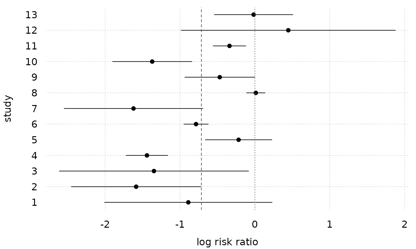
The picture explains the large tau. Studies 8 and 11
have short intervals that stay above the pooled line, and studies 4 and
10 have short intervals that stay below it. No single effect size can
hold all 13, so the random-effect term takes up the difference.
confint_varcorr(fmeta)
#>       block        term type  estimate       lwr       upr
#> 1 1 | study (Intercept)   sd 0.5596814 0.3310656 0.9461668
Cross-check against metafor
metafor::rma() is the reference implementation of this
model, and it uses REML by default.
rr <- metafor::rma(yi, vi, data = bcg, method = "REML")
out <- rbind(frmtmb = c(unname(fixef_by_dpar(fmeta)$mu),
                        sqrt(vcov(fmeta)[1, 1]),
                        VarCorr(fmeta)$study$sd["Intercept", "Estimate"]),
             metafor = c(as.numeric(rr$beta), rr$se, sqrt(rr$tau2)))
colnames(out) <- c("pooled_logRR", "se", "tau")
out
#>         pooled_logRR        se       tau
#> frmtmb    -0.7145323 0.1804360 0.5596814
#> metafor   -0.7145323 0.1797815 0.5596815
stopifnot(
  abs(fixef_by_dpar(fmeta)$mu - as.numeric(rr$beta)) < 1e-5,
  abs(VarCorr(fmeta)$study$sd["Intercept", "Estimate"] -
        sqrt(rr$tau2)) < 1e-5,
  # the standard errors come from different expressions: metafor uses
  # (X'WX)^-1 at the REML tau, frmtmb reads the joint Hessian
  abs(sqrt(vcov(fmeta)[1, 1]) / rr$se - 1) < 0.01
)
The pooled estimate and the heterogeneity match to five decimal places. The standard errors agree to under one percent, because the two packages compute them from different expressions.
Meta-regression
Adding a moderator makes it a meta-regression. Absolute latitude is the classic moderator for these trials: the vaccine works better away from the equator.
freg <- frm(bf(yi | se(sei) ~ ablat + (1 | study)) + gaussian(),
            data = bcg, REML = TRUE)
c(fixef_by_dpar(freg)$mu, tau = VarCorr(freg)$study$sd["Intercept", "Estimate"])
#> (Intercept)       ablat         tau
#>  0.25146821 -0.02910173  0.27631135
rr2 <- metafor::rma(yi, vi, mods = ~ablat, data = bcg, method = "REML")
out <- rbind(frmtmb = c(fixef_by_dpar(freg)$mu,
                        VarCorr(freg)$study$sd["Intercept", "Estimate"]),
             metafor = c(coef(rr2), sqrt(rr2$tau2)))
colnames(out) <- c("intercept", "ablat", "tau")
out
#>         intercept       ablat       tau
#> frmtmb  0.2514682 -0.02910173 0.2763114
#> metafor 0.2514643 -0.02910166 0.2763235
Latitude removes about half of the heterogeneity: tau
falls from 0.56 to 0.28.
Because this is an ordinary mixed model with a fixed residual, the
rest of the grammar still applies. Nested study levels become a second
grouping factor, which is the multilevel meta-analysis. A formula on
sigma turns the fixed residual into a modeled one, which is
se(sei, sigma = TRUE) in brms.
4. Monotonic effects of ordinal predictors
An ordinal predictor such as an income band or a Likert item is
neither a number nor an unordered factor. Treating it as a number forces
equal steps. Treating it as a factor throws the order away.
mo() keeps the order and estimates the step sizes as a
simplex, which is the method of Bürkner and Charpentier (2020,
British Journal of Mathematical and Statistical Psychology 73),
and the subject of the brms monotonic effects vignette.
set.seed(21)
n <- 400; L <- 6
inc <- sample(1:L, n, TRUE)
shape <- c(0, 0.15, 0.3, 0.75, 0.9, 1)   # a step between bands 3 and 4
dmo <- data.frame(income = factor(inc, ordered = TRUE), z = rnorm(n))
dmo$ls <- 5 + 2.0 * shape[inc] + 0.4 * dmo$z + rnorm(n, 0, 0.8)
fmo <- frm(bf(ls ~ mo(income) + z) + gaussian(), data = dmo)
fixef_by_dpar(fmo)$mu
#> (Intercept)           z    moincome
#>   5.1896894   0.4225085   0.3610907
moincome is the average step, not the total effect. The
total effect across the whole scale is moincome * (L - 1),
here about 1.8. To read the shape, predict at each band with the other
predictors held fixed and rescale to the unit interval.
nd <- data.frame(income = factor(1:L, ordered = TRUE), z = 0)
p <- frm_linpred(fmo, newdata = nd)
rbind(estimated = round((p - p[1]) / (p[L] - p[1]), 3),
      simulated = shape)
#>           1     2     3    4     5 6
#> estimated 0 0.112 0.276 0.85 0.896 1
#> simulated 0 0.150 0.300 0.75 0.900 1
The fit finds the large step between bands 3 and 4 and the small steps elsewhere.
Cross-check against the saturated factor model
mo() is the saturated factor model with an order
restriction, and it spends the same number of parameters. When the band
means already increase, the restriction is not active and the two fits
are identical.
fsat <- frm(bf(ls ~ income + z) + gaussian(), data = dmo)
out <- rbind(
  mo = c(frm_linpred(fmo, newdata = nd), logLik(fmo), attr(logLik(fmo), "df")),
  saturated = c(frm_linpred(fsat, newdata = nd), logLik(fsat),
                attr(logLik(fsat), "df")))
colnames(out) <- c(paste0("band", 1:L), "logLik", "df")
round(out, 4)
#>            band1  band2  band3  band4  band5  band6    logLik df
#> mo        5.1897 5.3915 5.6879 6.7237 6.8077 6.9951 -481.0059  8
#> saturated 5.1897 5.3915 5.6879 6.7237 6.8077 6.9951 -481.0059  8
stopifnot(max(abs(frm_linpred(fmo, newdata = nd) -
                    frm_linpred(fsat, newdata = nd))) < 1e-4)
The step shape is easier to read as a picture than as a row of
numbers. The points are the observed band means with 95 percent
intervals, the line is the mo() fit at z = 0,
and the crosses are the saturated factor fit at the same place.
band <- as.numeric(tapply(dmo$ls, dmo$income, mean))
band_se <- as.numeric(tapply(dmo$ls, dmo$income,
                             function(v) sd(v) / sqrt(length(v))))
tinyplot::tinyplot(x = 1:L, y = band, ymin = band - 1.96 * band_se,
                   ymax = band + 1.96 * band_se, type = "pointrange",
                   theme = "clean2", col = "gray20", pch = 16,
                   xlab = "income band", ylab = "mean of ls")
tinyplot::plt_add(x = 1:L, y = as.numeric(p), type = "l",
                  col = "firebrick", lwd = 2)
tinyplot::plt_add(x = 1:L, y = as.numeric(frm_linpred(fsat, newdata = nd)),
                  type = "p", pch = 4, cex = 1.6, col = "steelblue")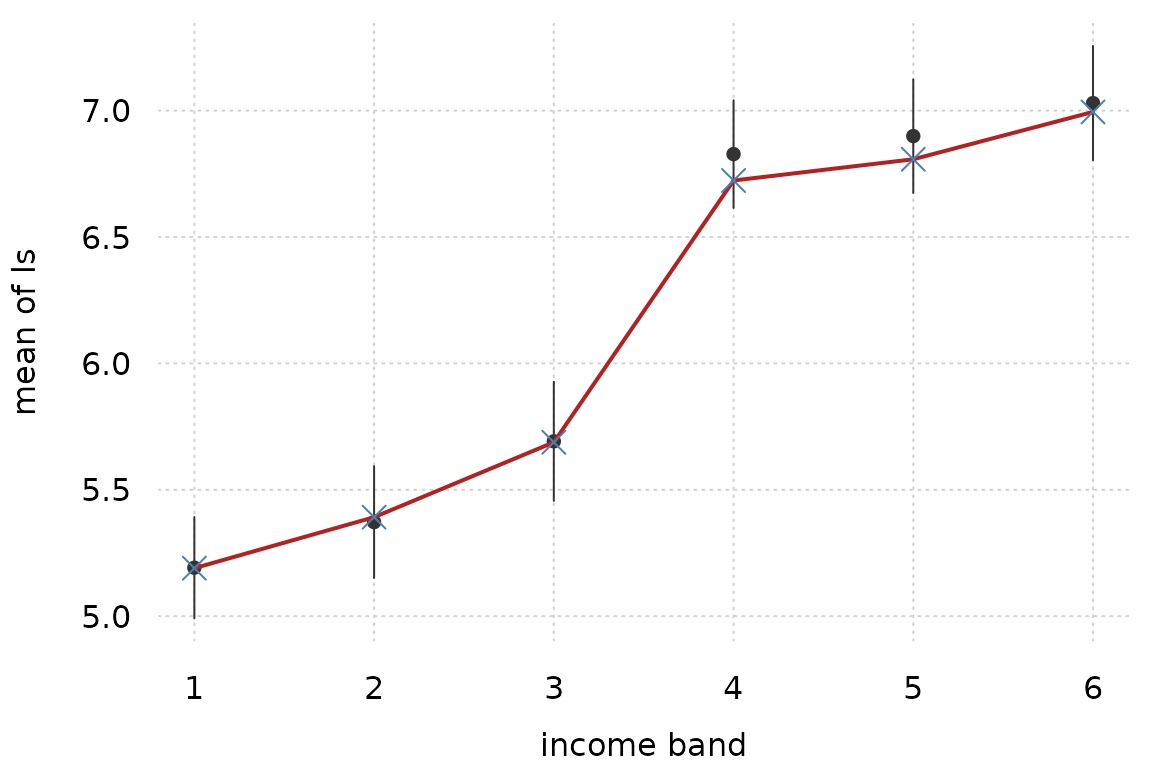
The big step between bands 3 and 4 is the shape the simulation put there, and the two fits are the same curve.
The value of mo() is not the parameter count. It is that
one coefficient carries the effect size, that the restriction holds when
the data are noisy, and that interactions stay readable.
mo() takes two-way interactions with numeric terms.
fixef_by_dpar(frm(bf(ls ~ mo(income) * z) + gaussian(),
                  data = dmo))$mu
#> (Intercept)           z    moincome  moincome:z
#>  5.19029028  0.29103078  0.36016768  0.03601463
The interaction is near zero here, which is right: the simulation has no interaction. A factor multiplier is refused, so expand a factor into numeric indicator columns first.
5. Location-scale regression
GAMLSS calls it a location-scale model, mgcv calls it
gaulss, and brms calls it distributional regression. The
mean and the residual standard deviation both follow smooth functions of
a covariate. In frmtmb this is one bf() with a formula for
sigma, and the smoothing parameters of both smooths are
estimated as variance components.
set.seed(22)
dls <- data.frame(x = runif(400))
dls$y <- rnorm(400, sin(2 * pi * dls$x),
               exp(-1 + 1.2 * cos(2 * pi * dls$x)))
fls <- frm(bf(y ~ s(x, k = 10), sigma ~ s(x, k = 10)) + gaussian(),
           data = dls)
confint_varcorr(fls)
#>         block       term type estimate      lwr      upr
#> 1        s(x) sd(wiggle)   sd 2.302052 1.313378 4.034970
#> 2 sigma: s(x) sd(wiggle)   sd 2.465578 1.319760 4.606196
The two standard deviations are the smooths’ wiggliness parameters. A value near zero would mean a straight line.
Cross-check against mgcv
mgcv::gam() with family = gaulss() and
method = "ML" fits the same model. It uses a
logb link for the precision, so its scale parameterization
differs slightly from the plain log link here.
gm <- mgcv::gam(list(y ~ s(x, k = 10), ~ s(x, k = 10)), data = dls,
                family = mgcv::gaulss(b = 0), method = "ML")
nd <- data.frame(x = seq(0.05, 0.95, length.out = 6))
pg <- predict(gm, newdata = nd, type = "response")
out <- rbind(frmtmb_mu = frm_linpred(fls, newdata = nd),
             mgcv_mu = pg[, 1],
             frmtmb_sigma = frm_linpred(fls, newdata = nd, dpar = "sigma",
                                    type = "response"),
             mgcv_sigma = 1 / pg[, 2],
             true_sigma = exp(-1 + 1.2 * cos(2 * pi * nd$x)))
colnames(out) <- paste0("x=", round(nd$x, 2))
round(out, 4)
#>              x=0.05 x=0.23 x=0.41  x=0.59  x=0.77  x=0.95
#> frmtmb_mu    0.5197 1.0491 0.5352 -0.5705 -0.9096 -0.7964
#> mgcv_mu      0.5115 1.0497 0.5350 -0.5707 -0.9072 -0.7978
#> frmtmb_sigma 1.1933 0.3860 0.1338  0.1487  0.4431  1.1790
#> mgcv_sigma   1.1720 0.3804 0.1315  0.1463  0.4379  1.1597
#> true_sigma   1.1517 0.4276 0.1336  0.1336  0.4276  1.1517
sg <- frm_linpred(fls, newdata = nd, dpar = "sigma", type = "response")
stopifnot(
  max(abs(frm_linpred(fls, newdata = nd) - pg[, 1])) < 0.02,
  max(abs(sg * pg[, 2] - 1)) < 0.03
)
The two mean curves agree to about 0.01, and the two scale curves to
about two percent. They are not expected to agree exactly, because the
packages choose their smoothing parameters with different criteria. Note
that frm_linpred() on a distributional parameter returns
the link scale by default, so type = "response" is needed
for a standard deviation.
One figure holds both curves. The band is the frmtmb mean plus and minus two fitted standard deviations, so its center is the location model and its width is the scale model. The dashed lines are the same band from mgcv.
xg <- data.frame(x = seq(0, 1, length.out = 100))
mu_f <- as.numeric(frm_linpred(fls, newdata = xg))
sd_f <- as.numeric(frm_linpred(fls, newdata = xg, dpar = "sigma",
                           type = "response"))
pg <- predict(gm, newdata = xg, type = "response")
tinyplot::tinyplot(x = xg$x, y = mu_f, ymin = mu_f - 2 * sd_f,
                   ymax = mu_f + 2 * sd_f, type = "ribbon",
                   theme = "clean2", xlab = "x", ylab = "y",
                   ylim = range(dls$y))
tinyplot::plt_add(x = dls$x, y = dls$y, type = "p", pch = 16, cex = 0.5,
                  col = "gray45")
lines(xg$x, mu_f, lwd = 2, col = "steelblue4")
lines(xg$x, pg[, 1] - 2 / pg[, 2], lty = 2, col = "firebrick")
lines(xg$x, pg[, 1] + 2 / pg[, 2], lty = 2, col = "firebrick")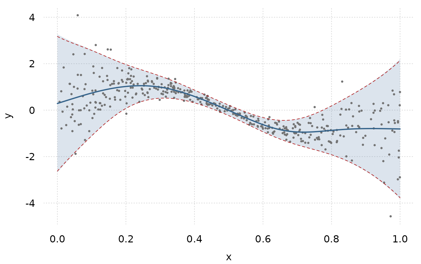
The band is narrow where cos(2 pi x) is smallest, near
x = 0.5, and it opens at both ends. A constant-variance
smooth would draw a band of one width and would miss both. The mgcv
lines sit on the edges of the frmtmb band, which is the agreement of the
table above, drawn.
6. Growth mixture models
A growth mixture model says that a population contains latent classes
with different trajectories, and that individuals inside a class still
vary. It comes from the structural equation modeling literature (Muthen
and Shedden 1999, Biometrics 55), and brms fits it with
mixture(..., groups = ~id).
The groups argument is what makes it a growth mixture
rather than an observation-level mixture. Without it, every measurement
could belong to a different class. With it, the class is drawn once per
subject, so all of a subject’s measurements come from the same
component.
set.seed(31)
nid <- 80; nt <- 5
cls <- rbinom(nid, 1, 0.4)              # class membership per subject
id <- rep(seq_len(nid), each = nt)
dg <- data.frame(id = factor(id), time = rep(0:(nt - 1), nid))
b0 <- 2 + rnorm(nid, 0, 0.5)            # random intercept inside class
b1 <- c(0.2, 1.2)[cls + 1]              # slow and fast classes
dg$y <- b0[id] + b1[id] * dg$time + rnorm(nid * nt, 0, 0.6)
fgmm <- frm(bf(y ~ time + (1 | id)) +
              mixture(gaussian(), gaussian(), groups = ~id),
            data = dg)
rbind(class1 = fixef_by_dpar(fgmm)$mu1, class2 = fixef_by_dpar(fgmm)$mu2)
#>        (Intercept)     time
#> class1    1.981932 0.227937
#> class2    2.006057 1.258254
Each component keeps its own intercept, slope, residual standard deviation, and random intercept. The two slopes recover the slow and fast trajectories.
mixture_probs() gives the posterior class probability of
each subject.
pr <- mixture_probs(fgmm)
head(round(pr, 3), 3)
#>   class1 class2
#> 1      1      0
#> 2      0      1
#> 3      1      0
assigned <- max.col(pr) - 1L
# label switching is inherent to a mixture, so score both labelings
max(mean(assigned == cls), mean(assigned != cls))
#> [1] 1
Every subject is classified correctly here, because the two trajectories separate well over five time points. Real growth mixture models are rarely this clean.
Split the subject trajectories by the class the model gives them, and draw each component mean over its own panel.
dg$class <- factor(assigned[as.integer(dg$id)] + 1L,
                   labels = c("class 1", "class 2"))
tt <- 0:(nt - 1)
b <- rbind(fixef_by_dpar(fgmm)$mu1, fixef_by_dpar(fgmm)$mu2)
comp <- data.frame(
  time = rep(tt, 2),
  yhat = c(b[1, 1] + b[1, 2] * tt, b[2, 1] + b[2, 2] * tt),
  class = factor(rep(c("class 1", "class 2"), each = length(tt))))
tinyplot::tinyplot(y ~ time | id, data = dg, facet = ~class, type = "l",
                   col = "gray60", legend = FALSE, theme = "clean2",
                   xlab = "time", ylab = "y")
tinyplot::plt_add(yhat ~ time, data = comp, facet = ~class, type = "l",
                  col = "black", lwd = 3)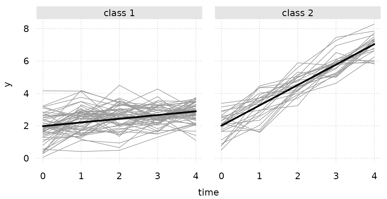
The two panels are the model’s answer to the question the mixture asks. Inside a panel the lines are near parallel, which is the random intercept. Between panels the lines differ in slope, which is the class.
Two cautions carry over from any maximum likelihood mixture. The
likelihood is multimodal, so compare starting values with
frm_allfit(). And a mixture will always find classes,
whether or not they exist, so a model comparison against the
single-class fit is the minimum evidence for reporting them.
7. Measurement error in a predictor
When a predictor is measured with error, regression on the measured
value is biased toward zero. The bias factor is the reliability ratio,
var(true) / (var(true) + sd_error^2). brms corrects it by
giving the mismeasured variable its own sub-model with a known error
standard deviation, spelled mi(sdx) on that response and
mi(x) in the predictor of interest. frmtmb uses the same
spelling and integrates the latent true values out with the Laplace
approximation.
set.seed(3)
n <- 300
z <- rnorm(n)
x_true <- rnorm(n, 0.5 * z, 1)
su <- 0.6                                # known measurement error sd
dme <- data.frame(x = x_true + rnorm(n, 0, su), z = z, su = su)
dme$y <- 1 + 1.0 * x_true + 0.3 * z + rnorm(n, 0, 0.7)
fme <- frm(bf(y ~ mi(x) + z) + gaussian() +
             bf(x | mi(su) ~ z) + gaussian(),
           data = dme)
fixef_by_dpar(fme)$y_mu
#> (Intercept)           z         mix
#>   0.9701412   0.3316033   1.0379552
The coefficient on the latent x is mix.
Compare it with the naive regression on the measured value, and with the
attenuation that theory predicts.
naive <- coef(lm(y ~ x + z, data = dme))[["x"]]
c(naive = naive,
  predicted_attenuation = 1.0 * var(x_true) / (var(x_true) + su^2),
  corrected = fixef_by_dpar(fme)$y_mu[["mix"]],
  simulated_truth = 1.0)
#>                 naive predicted_attenuation             corrected
#>             0.7703484             0.7855849             1.0379552
#>       simulated_truth
#>             1.0000000
stopifnot(fixef_by_dpar(fme)$y_mu[["mix"]] > naive + 0.1)
The naive slope sits near the attenuated value that theory predicts. The corrected slope is close to the truth. The correction is not free: it widens the standard error, because the latent values are estimated rather than observed.
c(naive_se = summary(lm(y ~ x + z, data = dme))$coefficients["x", 2],
  corrected_se = sqrt(diag(vcov(fme)))[["y_mix"]])
#>     naive_se corrected_se
#>   0.04373838   0.06561273
The same machinery with mi() and no standard deviation
imputes missing values in one step instead of correcting known
error.
8. Sequential ordinal models with category-specific effects
The proportional odds assumption says one slope governs every
category threshold. cs() relaxes it and gives each
threshold its own slope, which is brms’s category-specific effect. Under
the cumulative parameterization that model can produce negative
probabilities, so brms and frmtmb both refuse it there and accept it for
the sequential families sratio, cratio, and
acat.
set.seed(51)
n <- 500
xo <- rnorm(n)
th <- c(-1.6, 0, 1.6); eff <- c(0.3, 0.6, 0.9)
Y <- integer(n)
for (i in seq_len(n)) {
  cp <- c(plogis(th - eff * xo[i]), 1)
  Y[i] <- sample(1:4, 1, prob = diff(c(0, cp)))
}
dord <- data.frame(y = factor(Y, ordered = TRUE), x = xo)
fcs <- frm(bf(y ~ cs(x)) + sratio(), data = dord)
confint(fcs)
#>                      lwr        upr        est
#> Intercept[1] -1.56199949 -1.1273864 -1.3446929
#> Intercept[2] -0.67583509 -0.2497143 -0.4627747
#> Intercept[3]  0.76770573  1.4194112  1.0935585
#> x[1]         -0.07596909  0.3784586  0.1512448
#> x[2]          0.47728372  0.9677452  0.7225145
#> x[3]          0.40132773  1.0910094  0.7461686
The rows Intercept[k] are the thresholds themselves:
sratio() does not order them, as brms does not. The rows
x[k] are the effect of x at threshold
k. The three effects grow, which is what the simulation put
there.
Cross-check against a set of binomial regressions
The sequential model has an exact decomposition. It asks, at each
category in turn, whether the process stops there given that it reached
there. Those questions are independent, so the model is equivalent to
K - 1 separate logistic regressions on shrinking subsets,
and the log likelihoods add up (Laara and Matthews 1985,
Biometrika 72; Tutz 1991).
glm_fits <- lapply(1:3, function(k) {
  sub <- dord[as.integer(dord$y) >= k, ]
  glm(as.integer(as.integer(sub$y) == k) ~ x, data = sub,
      family = binomial())
})
rbind(frmtmb = confint(fcs)[paste0("x[", 1:3, "]"), "est"],
      # the binary question is "stop here", so the sign is reversed
      binomial_glms = -vapply(glm_fits, function(g) coef(g)[["x"]], 0))
#>                    x[1]      x[2]      x[3]
#> frmtmb        0.1512448 0.7225145 0.7461686
#> binomial_glms 0.1512442 0.7225128 0.7461606
c(frmtmb = as.numeric(logLik(fcs)),
  sum_of_glms = sum(vapply(glm_fits, function(g) as.numeric(logLik(g)), 0)))
#>      frmtmb sum_of_glms
#>   -638.4767   -638.4767
stopifnot(
  max(abs(confint(fcs)[paste0("x[", 1:3, "]"), "est"] +
            vapply(glm_fits, function(g) coef(g)[["x"]], 0))) < 1e-4,
  abs(as.numeric(logLik(fcs)) -
        sum(vapply(glm_fits, function(g) as.numeric(logLik(g)), 0))) < 1e-6
)
The coefficients and the log likelihood agree exactly. The frmtmb form is the more general one, because the decomposition breaks as soon as a random effect is shared between thresholds, and frmtmb keeps working.
A proportional odds fit is the null model, and anova()
tests the restriction.
anova(frm(bf(y ~ x) + sratio(), data = dord), fcs)
#> Likelihood-ratio tests
#> Each test assumes the smaller model is nested in the larger; see ?anova.frmtmb_fit
#>
#>           Df  logLik    AIC  Chisq Chi Df Pr(>Chisq)
#> y ~ x      4 -645.57 1299.1
#> y ~ cs(x)  6 -638.48 1289.0 14.187      2  0.0008305 ***
#> ---
#> Signif. codes:  0 '***' 0.001 '**' 0.01 '*' 0.05 '.' 0.1 ' ' 1
9. Multivariate responses with correlated residuals
Two traits measured on the same animals are two responses, not one.
brms’s multivariate vignette opens with two morphological traits of blue
tit chicks, taken from MCMCglmm’s BTdata (Hadfield 2010,
Journal of Statistical Software 33(2)). Chicks share foster
nests, so a nest effect enters both traits. The traits are measured on
the same chick, so what is left over after the nest effect correlates
too. Drop the grouping factor and the model is Zellner’s seemingly
unrelated regressions (1962, Journal of the American Statistical
Association 57).
frmtmb writes this with one formula per response. mvbf()
collects them, the |ID| identifier ties the two grouping
blocks into a single covariance, and rescor = TRUE adds the
residual correlation across responses. Section 1 fits a two-trait model
the other way, in long format with the traits stacked into one response
column. This section uses the wide spelling.
The two correlations answer different questions. The
|ID| block asks whether nests that are heavy are also long.
rescor asks whether a chick that is heavy for its nest is
also long for its nest. Nothing makes the answers agree. Here they have
opposite signs, and the raw correlation of the two columns reports
neither of them.
set.seed(1)
n_nest <- 40L; per_nest <- 5L
n_bird <- n_nest * per_nest
nest <- factor(rep(seq_len(n_nest), each = per_nest))
age <- rnorm(n_bird)
# the nest effects correlate positively and the within-bird residuals
# negatively, so the two levels disagree by construction
Gt <- matrix(c(0.36, 0.162, 0.162, 0.2025), 2, 2)
St <- matrix(c(0.64, -0.24, -0.24, 0.36), 2, 2)
u <- matrix(rnorm(n_nest * 2), n_nest, 2) %*% chol(Gt)
e <- matrix(rnorm(n_bird * 2), n_bird, 2) %*% chol(St)
bt <- data.frame(
  nest = nest, age = age,
  mass = 1 + 0.5 * age + u[as.integer(nest), 1] + e[, 1],
  tarsus = -0.5 + 0.9 * age + u[as.integer(nest), 2] + e[, 2])
c(raw_correlation = cor(bt$mass, bt$tarsus),
  correlation_of_nest_means = cor(tapply(bt$mass, bt$nest, mean),
                                  tapply(bt$tarsus, bt$nest, mean)))
#>           raw_correlation correlation_of_nest_means
#>                 0.2345493                 0.2976839
The fit
fbt <- frm(mvbf(bf(mass ~ age + (1 | p | nest)),
                bf(tarsus ~ age + (1 | p | nest)), rescor = TRUE) +
             gaussian(), data = bt)
confint_varcorr(fbt)
#>                                  block
#> 1 mass 1 | nest + tarsus 1 | nest [ID]
#> 2 mass 1 | nest + tarsus 1 | nest [ID]
#> 3 mass 1 | nest + tarsus 1 | nest [ID]
#>                                             term type  estimate        lwr
#> 1                            mass.mu:(Intercept)   sd 0.5874726 0.43339096
#> 2                          tarsus.mu:(Intercept)   sd 0.4787523 0.35364102
#> 3 cor(mass.mu:(Intercept),tarsus.mu:(Intercept))  cor 0.5273159 0.03750564
#>         upr
#> 1 0.7963341
#> 2 0.6481254
#> 3 0.8128310
rescor_matrix(fbt)
#>              mass     tarsus
#> mass    1.0000000 -0.4466081
#> tarsus -0.4466081  1.0000000
p is the |ID| label. It is an arbitrary
name, and the only thing it does is say that these two bar terms are one
block. One 2 by 2 covariance comes back for it, so
confint_varcorr() reports two standard deviations and the
correlation between them. rescor_matrix() reports the
residual correlation, which is a separate matrix because it describes a
different level.
Gh <- VarCorr(fbt)$nest$cov[, "Estimate", ]
out <- rbind(
  estimated = c(sqrt(diag(Gh)), cov2cor(Gh)[1, 2], sigma(fbt),
                rescor_matrix(fbt)[1, 2]),
  simulated = c(sqrt(diag(Gt)), cov2cor(Gt)[1, 2], sqrt(diag(St)),
                cov2cor(St)[1, 2]))
colnames(out) <- c("sd_nest_mass", "sd_nest_tarsus", "cor_nest",
                   "sigma_mass", "sigma_tarsus", "rescor")
round(out, 3)
#>           sd_nest_mass sd_nest_tarsus cor_nest sigma_mass sigma_tarsus rescor
#> estimated        0.587          0.479    0.527      0.801        0.648 -0.447
#> simulated        0.600          0.450    0.600      0.800        0.600 -0.500
Both correlations come back with the sign and the rough size the simulation put there. Neither is the raw correlation of the columns printed above, which sits between them and matches neither level.
Cross-check against the closed-form marginal likelihood
This model needs no random effects to write down. Within one nest,
stack both traits and the result is a multivariate normal whose
covariance is S %x% I + G %x% J, where S is
the residual matrix, G is the nest matrix, I
is the identity and J is a matrix of ones. Nests are
independent, so their log densities add. optim() maximizes
that sum with the regression coefficients profiled out by generalized
least squares. It uses no part of frmtmb.
Xj <- lapply(levels(bt$nest), function(g)
  kronecker(diag(2), cbind(1, bt$age[bt$nest == g])))
yj <- lapply(levels(bt$nest), function(g)
  c(bt$mass[bt$nest == g], bt$tarsus[bt$nest == g]))
nll <- function(p) {
  Lg <- matrix(c(exp(p[1]), p[2], 0, exp(p[3])), 2, 2)
  Gp <- tcrossprod(Lg)
  s <- exp(p[4:5]); rho <- tanh(p[6])
  Sp <- outer(s, s) * matrix(c(1, rho, rho, 1), 2, 2)
  V <- kronecker(Sp, diag(per_nest)) +
    kronecker(Gp, matrix(1, per_nest, per_nest))
  Vi <- solve(V)
  M <- Reduce(`+`, lapply(Xj, function(X) crossprod(X, Vi %*% X)))
  b <- solve(M, Reduce(`+`, Map(function(X, y) crossprod(X, Vi %*% y),
                                Xj, yj)))
  q <- sum(vapply(seq_along(yj), function(j) {
    r <- yj[[j]] - Xj[[j]] %*% b; sum(r * (Vi %*% r))
  }, 0))
  as.numeric(0.5 * (2 * n_bird * log(2 * pi) +
                      n_nest * determinant(V)$modulus + q))
}
# bounds, because an unbounded step can send the two scales far enough
# apart to make V numerically singular before the optimizer recovers
op <- optim(c(log(0.5), 0.1, log(0.5), log(0.8), log(0.6), atanh(-0.4)),
            nll, method = "L-BFGS-B", lower = rep(-6, 6),
            upper = rep(6, 6),
            control = list(factr = 1e-2, pgtol = 0, maxit = 2000))
Gc <- tcrossprod(matrix(c(exp(op$par[1]), op$par[2], 0, exp(op$par[3])),
                        2, 2))
out <- rbind(
  frmtmb = c(sqrt(diag(Gh)), cov2cor(Gh)[1, 2], sigma(fbt),
             rescor_matrix(fbt)[1, 2], as.numeric(logLik(fbt))),
  closed_form = c(sqrt(diag(Gc)), cov2cor(Gc)[1, 2], exp(op$par[4:5]),
                  tanh(op$par[6]), -op$value))
colnames(out) <- c("sd_nest_mass", "sd_nest_tarsus", "cor_nest",
                   "sigma_mass", "sigma_tarsus", "rescor", "logLik")
round(out, 6)
#>             sd_nest_mass sd_nest_tarsus cor_nest sigma_mass sigma_tarsus
#> frmtmb          0.587473       0.478752 0.527316   0.801149     0.647952
#> closed_form     0.587471       0.478752 0.527320   0.801149     0.647952
#>                rescor    logLik
#> frmtmb      -0.446608 -469.6262
#> closed_form -0.446608 -469.6262
stopifnot(
  abs(as.numeric(logLik(fbt)) + op$value) < 1e-6,
  max(abs(out["frmtmb", 1:6] - out["closed_form", 1:6])) < 1e-4
)
The log likelihood agrees to under 1e-6 and every variance parameter to under 1e-4. The Laplace approximation is exact for a gaussian response, so the only thing that separates the two numbers is optimizer noise.
What each correlation buys
Turn both correlations off and the multivariate fit is two univariate fits standing next to each other. That is the cheapest reference there is, and it is exact: the log likelihoods add.
fnone <- frm(mvbf(bf(mass ~ age + (1 | nest)),
                  bf(tarsus ~ age + (1 | nest))) + gaussian(), data = bt)
u1 <- frm(bf(mass ~ age + (1 | nest)) + gaussian(), data = bt)
u2 <- frm(bf(tarsus ~ age + (1 | nest)) + gaussian(), data = bt)
fid <- frm(mvbf(bf(mass ~ age + (1 | p | nest)),
                bf(tarsus ~ age + (1 | p | nest))) + gaussian(), data = bt)
c(two_separate_fits = as.numeric(logLik(u1)) + as.numeric(logLik(u2)),
  uncoupled_mvbf = as.numeric(logLik(fnone)),
  plus_ID = as.numeric(logLik(fid)),
  plus_rescor = as.numeric(logLik(fbt)))
#> two_separate_fits    uncoupled_mvbf           plus_ID       plus_rescor
#>         -488.7960         -488.7960         -487.3920         -469.6262
stopifnot(abs(as.numeric(logLik(fnone)) - as.numeric(logLik(u1)) -
                as.numeric(logLik(u2))) < 1e-6)
c(uncoupled = AIC(fnone), plus_ID = AIC(fid), plus_rescor = AIC(fbt))
#>   uncoupled     plus_ID plus_rescor
#>    993.5921    992.7840    959.2523
Each correlation costs one parameter. The |ID|
correlation pays for itself by a little and the residual correlation by
a lot. That order is the one the design implies: the nest correlation
rests on one pair of effects per nest, and the residual correlation on
one pair per chick.
What rescor does not buy here is precision on the
regression coefficients.
rbind(with_rescor = sqrt(diag(vcov(fbt)))[1:4],
      without = sqrt(diag(vcov(fid)))[1:4])
#>             mass_Intercept tarsus_Intercept   mass_age tarsus_age
#> with_rescor      0.1088242       0.08850337 0.06550657 0.05299467
#> without          0.1089673       0.08862100 0.06605197 0.05343918
The standard errors barely move, and Zellner’s result says why. When
every equation carries the same predictors, correlating the errors
leaves the coefficients exactly where equation-by-equation least squares
puts them. The shared nest block stops that identity from being exact
here, and what survives of it is a difference too small to report. The
gain from rescor shows up when the equations carry
different predictors, and, more often, in the correlation itself, which
is usually the estimand rather than a nuisance. Section 1 reads a
genetic correlation the same way.
Reading residuals off a multivariate fit
residuals() refuses a multivariate fit, and says so.
residuals(fbt)
#> , , mass
#>
#>            Estimate Est.Error        Q2.5        Q97.5
#>   [1,]  0.292625468 0.2815784 -0.25925802  0.844508956
#>   [2,] -0.345655126 0.2774229 -0.88939393  0.198083682
#>   [3,]  1.031915370 0.2842553  0.47478520  1.589045542
#>   [4,] -0.569732925 0.2938941 -1.14575474  0.006288888
#>   [5,] -0.482998993 0.2777472 -1.02737359  0.061375607
#>   [6,] -0.753888513 0.2926816 -1.32753390 -0.180243127
#>   [7,] -0.477488885 0.2888063 -1.04353890  0.088561130
#>   [8,]  0.815136537 0.2909554  0.24487441  1.385398668
#>   [9,]  0.404696975 0.2894585 -0.16263130  0.972025246
#>  [10,]  0.855068219 0.2881367  0.29033075  1.419805685
#>  [11,] -0.292222938 0.3034875 -0.88704760  0.302601721
#>  [12,]  0.312317332 0.2883084 -0.25275680  0.877391462
#>  [13,]  0.198756902 0.2903117 -0.37024349  0.767757292
#>  [14,] -1.149867553 0.3223612 -1.78168381 -0.518051293
#>  [15,]  1.439632548 0.2962888  0.85891713  2.020347965
#>  [16,]  0.068147002 0.2842827 -0.48903688  0.625330882
#>  [17,]  0.573289703 0.2842035  0.01626114  1.130318271
#>  [18,]  0.732322295 0.2886872  0.16650571  1.298138882
#>  [19,] -0.073185052 0.2873528 -0.63638621  0.490016103
#>  [20,] -0.279137616 0.2854608 -0.83863059  0.280355358
#>  [21,]  0.043639878 0.2867379 -0.51835611  0.605635862
#>  [22,] -1.510192740 0.2852899 -2.06935069 -0.951034792
#>  [23,]  0.899259838 0.2822610  0.34603846  1.452481214
#>  [24,] -1.000629940 0.3149644 -1.61794887 -0.383311006
#>  [25,]  0.649710498 0.2839300  0.09321800  1.206203000
#>  [26,]  1.562755457 0.3152610  0.94485532  2.180655595
#>  [27,]  0.418589391 0.3147275 -0.19826519  1.035443978
#>  [28,]  0.795854335 0.3203149  0.16804863  1.423660038
#>  [29,] -0.469907549 0.3139271 -1.08519332  0.145378222
#>  [30,]  0.615045905 0.3196172 -0.01139231  1.241484116
#>  [31,]  1.099635313 0.2998460  0.51194787  1.687322752
#>  [32,]  0.332739241 0.2839918 -0.22387441  0.889352888
#>  [33,] -0.106051305 0.2858568 -0.66632028  0.454217667
#>  [34,] -0.270771341 0.2840153 -0.82743104  0.285888355
#>  [35,]  0.214913021 0.2958712 -0.36498385  0.794809893
#>  [36,]  0.943256935 0.2788342  0.39675202  1.489761849
#>  [37,] -0.299092531 0.2786673 -0.84527037  0.247085304
#>  [38,] -0.006137782 0.2768781 -0.54880898  0.536533418
#>  [39,] -0.935702415 0.2839991 -1.49233049 -0.379074341
#>  [40,]  0.492462520 0.2798324 -0.05599888  1.040923918
#>  [41,]  0.875691780 0.2801530  0.32660191  1.424781648
#>  [42,]  1.026318370 0.2803336  0.47687453  1.575762208
#>  [43,]  0.487775392 0.2846353 -0.07009947  1.045650250
#>  [44,] -1.660899633 0.2831444 -2.21585252 -1.105946746
#>  [45,]  0.210951986 0.2829531 -0.34362599  0.765529957
#>  [46,]  0.312935226 0.2848599 -0.24537987  0.871250322
#>  [47,] -0.326427050 0.2789480 -0.87315513  0.220301026
#>  [48,]  0.095799489 0.2812732 -0.45548594  0.647084913
#>  [49,] -0.738613021 0.2794222 -1.28627057 -0.190955478
#>  [50,]  0.503660558 0.2823600 -0.04975491  1.057076026
#>  [51,] -0.217115979 0.2792801 -0.76449491  0.330262955
#>  [52,] -1.218489714 0.2833276 -1.77380167 -0.663177755
#>  [53,] -0.249835174 0.2790927 -0.79684691  0.297176562
#>  [54,]  1.124334964 0.2912588  0.55347816  1.695191765
#>  [55,] -0.214880347 0.2911121 -0.78544967  0.355688979
#>  [56,]  0.508596941 0.3029349 -0.08514449  1.102338367
#>  [57,]  0.661563681 0.2793989  0.11395190  1.209175462
#>  [58,] -0.097405323 0.2879188 -0.66171572  0.466905077
#>  [59,] -0.370338230 0.2790378 -0.91724226  0.176565798
#>  [60,] -0.517671076 0.2780497 -1.06263850  0.027296347
#>  [61,]  0.759522104 0.3118100  0.14838568  1.370658532
#>  [62,] -0.701735863 0.2857709 -1.26183663 -0.141635099
#>  [63,]  0.351619665 0.2845300 -0.20604880  0.909288128
#>  [64,] -0.082050941 0.2853223 -0.64127236  0.477170478
#>  [65,] -1.668309984 0.2944109 -2.24534484 -1.091275130
#>  [66,] -1.411996979 0.2814233 -1.96357655 -0.860417404
#>  [67,]  0.432525690 0.3112032 -0.17742145  1.042472832
#>  [68,] -0.428095077 0.2929431 -1.00225295  0.146062794
#>  [69,]  0.357435930 0.2814517 -0.19419920  0.909071060
#>  [70,]  1.240359537 0.3090289  0.63467407  1.846044999
#>  [71,]  0.862726145 0.2946982  0.28512824  1.440324056
#>  [72,]  0.216295333 0.2907592 -0.35358217  0.786172833
#>  [73,] -0.011366038 0.2964395 -0.59237681  0.569644735
#>  [74,] -0.481486559 0.2923366 -1.05445574  0.091482620
#>  [75,]  0.932601783 0.2958333  0.35277914  1.512424423
#>  [76,]  0.908767349 0.2813960  0.35724129  1.460293408
#>  [77,] -0.512746815 0.2819750 -1.06540757  0.039913937
#>  [78,]  0.305027311 0.2806402 -0.24501742  0.855072041
#>  [79,] -1.105021819 0.2807096 -1.65520244 -0.554841199
#>  [80,]  0.268780136 0.2830682 -0.28602325  0.823583524
#>  [81,] -1.627324969 0.2853344 -2.18657014 -1.068079800
#>  [82,]  1.501081400 0.2836663  0.94510566  2.057057143
#>  [83,] -0.048428574 0.2956936 -0.62797739  0.531120246
#>  [84,]  0.095191190 0.2986563 -0.49016431  0.680546688
#>  [85,]  0.320047043 0.2872414 -0.24293584  0.883029928
#>  [86,]  0.258620650 0.2829021 -0.29585718  0.813098484
#>  [87,]  0.317148196 0.2867773 -0.24492492  0.879221309
#>  [88,]  0.218294956 0.2860863 -0.34242381  0.779013726
#>  [89,] -0.688902150 0.2829053 -1.24338633 -0.134417967
#>  [90,] -1.322294654 0.2829477 -1.87686195 -0.767727362
#>  [91,] -0.093850288 0.2891336 -0.66054165  0.472841076
#>  [92,]  0.452955480 0.2826222 -0.10097391  1.006884866
#>  [93,] -0.428206712 0.2821869 -0.98128281  0.124869386
#>  [94,]  0.171637071 0.2797282 -0.37662017  0.719894316
#>  [95,] -0.700583608 0.2872839 -1.26364965 -0.137517566
#>  [96,] -0.140189759 0.2843254 -0.69745729  0.417077768
#>  [97,] -0.044607915 0.2832252 -0.59971909  0.510503263
#>  [98,] -0.258969617 0.2775611 -0.80297930  0.285040064
#>  [99,] -0.278420204 0.2825535 -0.83221487  0.275374466
#> [100,]  1.269342512 0.2773686  0.72571010  1.812974924
#> [101,]  0.009812690 0.2844807 -0.54775917  0.567384550
#> [102,]  0.293996530 0.2825113 -0.25971549  0.847708547
#> [103,] -1.341062456 0.2874147 -1.90438497 -0.777739943
#> [104,] -0.462781097 0.2828506 -1.01715804  0.091595845
#> [105,]  0.323339786 0.2847617 -0.23478288  0.881462449
#> [106,]  0.407964251 0.2917738 -0.16390192  0.979830419
#> [107,] -1.258407804 0.2850446 -1.81708493 -0.699730678
#> [108,]  0.722449083 0.2850503  0.16376085  1.281137316
#> [109,] -1.081447611 0.2863484 -1.64268011 -0.520215108
#> [110,] -0.196410997 0.2906284 -0.76603228  0.373210283
#> [111,]  0.750738082 0.2847880  0.19256393  1.308912239
#> [112,]  0.185386469 0.2838208 -0.37089210  0.741665041
#> [113,]  0.580815603 0.3022888 -0.01165948  1.173290685
#> [114,] -0.063296837 0.2848922 -0.62167533  0.495081657
#> [115,] -0.393289475 0.2832286 -0.94840732  0.161828373
#> [116,] -0.943788295 0.2776086 -1.48789124 -0.399685349
#> [117,]  1.070554379 0.2772347  0.52718431  1.613924452
#> [118,] -0.167452936 0.2770606 -0.71048168  0.375575805
#> [119,] -0.769601460 0.2786364 -1.31571871 -0.223484211
#> [120,]  0.489501879 0.2767391 -0.05289677  1.031900525
#> [121,]  0.345079295 0.2882261 -0.21983356  0.909992146
#> [122,]  1.016307352 0.2939520  0.44017209  1.592442609
#> [123,] -0.994624594 0.2857483 -1.55468090 -0.434568288
#> [124,] -0.824650957 0.2855349 -1.38428906 -0.265012852
#> [125,] -0.844322362 0.2851191 -1.40314554 -0.285499187
#> [126,] -0.055156680 0.2902598 -0.62405552  0.513742156
#> [127,] -0.053997865 0.2851912 -0.61296236  0.504966629
#> [128,]  0.003041976 0.2852221 -0.55598303  0.562066985
#> [129,]  1.388074390 0.2876047  0.82437947  1.951769309
#> [130,] -0.320656853 0.2855162 -0.88025833  0.238944620
#> [131,] -0.369911527 0.2763739 -0.91159437  0.171771320
#> [132,]  0.457646990 0.2779686 -0.08716147  1.002455454
#> [133,]  0.844074750 0.2792966  0.29666344  1.391486063
#> [134,] -0.689237881 0.2912538 -1.26008474 -0.118391016
#> [135,] -0.463946606 0.2774774 -1.00779229  0.079899078
#> [136,]  0.232974190 0.2975370 -0.35018753  0.816135914
#> [137,]  0.637807431 0.2886372  0.07208885  1.203526011
#> [138,] -0.379080285 0.2885964 -0.94471886  0.186558285
#> [139,] -1.323098068 0.2888972 -1.88932621 -0.756869925
#> [140,]  1.192782892 0.2895349  0.62530488  1.760260901
#> [141,]  1.164687645 0.2941013  0.58825966  1.741115632
#> [142,] -0.527831684 0.2960405 -1.10806042  0.052397053
#> [143,] -0.033499131 0.2890450 -0.60001700  0.533018737
#> [144,] -1.379756135 0.2771677 -1.92299486 -0.836517406
#> [145,]  0.478566868 0.2809567 -0.07209807  1.029231802
#> [146,]  1.579229163 0.2790228  1.03235450  2.126103826
#> [147,] -0.998590018 0.3125584 -1.61119332 -0.385986713
#> [148,] -0.328379635 0.2764073 -0.87012793  0.213368655
#> [149,] -0.227718745 0.2861154 -0.78849459  0.333057102
#> [150,] -0.262414242 0.2930306 -0.83674362  0.311915131
#> [151,] -1.398897130 0.2869443 -1.96129760 -0.836496662
#> [152,]  0.624887840 0.2841419  0.06797988  1.181795801
#> [153,] -1.003630931 0.2840800 -1.56041750 -0.446844364
#> [154,]  0.197095983 0.2881298 -0.36762800  0.761819969
#> [155,]  0.687178560 0.2965383  0.10597416  1.268382955
#> [156,] -0.640658827 0.3089221 -1.24613504 -0.035182609
#> [157,]  0.247505573 0.3031580 -0.34667318  0.841684324
#> [158,] -0.499174475 0.3024948 -1.09205343  0.093704480
#> [159,] -1.002615256 0.3148375 -1.61968551 -0.385545000
#> [160,]  0.057688984 0.3184496 -0.56646074  0.681838712
#> [161,] -0.499087871 0.2877877 -1.06314147  0.064965729
#> [162,]  1.260949330 0.2872812  0.69788857  1.824010091
#> [163,] -0.161745642 0.2943217 -0.73860554  0.415114252
#> [164,]  0.533787420 0.2919785 -0.03847984  1.106054679
#> [165,]  0.004056054 0.2899466 -0.56422887  0.572340974
#> [166,] -1.842286383 0.3366391 -2.50208691 -1.182485851
#> [167,] -0.547714011 0.3187249 -1.17240328  0.076975256
#> [168,]  0.196876345 0.3379738 -0.46554017  0.859292858
#> [169,]  0.735471477 0.3178010  0.11259303  1.358349920
#> [170,] -1.325436272 0.3159512 -1.94468916 -0.706183382
#> [171,]  1.080954310 0.3081466  0.47699799  1.684910630
#> [172,] -0.188923840 0.2837411 -0.74504610  0.367198423
#> [173,] -0.304977116 0.2828838 -0.85941911  0.249464877
#> [174,] -0.951283236 0.2849235 -1.50972304 -0.392843433
#> [175,] -0.871889422 0.2874198 -1.43522182 -0.308557025
#> [176,]  0.190824777 0.2834128 -0.36465416  0.746303713
#> [177,]  0.559595825 0.2793000  0.01217784  1.107013811
#> [178,] -1.516277765 0.2933309 -2.09119576 -0.941359773
#> [179,] -0.649540628 0.2800473 -1.19842327 -0.100657985
#> [180,]  0.583958233 0.2811881  0.03283964  1.135076825
#> [181,] -0.370011095 0.3190037 -0.99524689  0.255224700
#> [182,]  1.741794201 0.3281831  1.09856722  2.385021187
#> [183,]  1.000206010 0.3176440  0.37763521  1.622776812
#> [184,]  0.466997848 0.3218884 -0.16389192  1.097887616
#> [185,]  0.009837899 0.3209084 -0.61913106  0.638806857
#> [186,] -0.295110251 0.2767158 -0.83746334  0.247242840
#> [187,] -1.070806720 0.2936957 -1.64643975 -0.495173694
#> [188,] -0.020868057 0.2806447 -0.57092163  0.529185512
#> [189,]  0.663479174 0.2777754  0.11904931  1.207909043
#> [190,]  0.342228229 0.2826047 -0.21166677  0.896123233
#> [191,] -0.295359449 0.2822058 -0.84847257  0.257753672
#> [192,] -0.935400151 0.2851213 -1.49422754 -0.376572764
#> [193,]  0.263234717 0.2841731 -0.29373428  0.820203715
#> [194,]  0.715715779 0.2904643  0.14641630  1.285015254
#> [195,]  1.428081601 0.2895144  0.86064379  1.995519414
#> [196,] -1.091640309 0.2832787 -1.64685629 -0.536424325
#> [197,]  0.273947910 0.2934769 -0.30125617  0.849151994
#> [198,]  0.150294944 0.2828143 -0.40401085  0.704600737
#> [199,]  0.929668753 0.2779371  0.38492206  1.474415442
#> [200,] -0.053938388 0.2767813 -0.59641976  0.488542984
#>
#> , , tarsus
#>
#>            Estimate Est.Error         Q2.5        Q97.5
#>   [1,] -0.170405459 0.2289189 -0.619078254  0.278267335
#>   [2,] -0.386275762 0.2253101 -0.827875372  0.055323848
#>   [3,] -0.519226198 0.2311404 -0.972253138 -0.066199258
#>   [4,]  0.027108082 0.2381517 -0.439660613  0.493876778
#>   [5,]  1.474414898 0.2255240  1.032395968  1.916433829
#>   [6,]  1.761486050 0.2370059  1.296963096  2.226009003
#>   [7,]  0.227337484 0.2327264 -0.228797920  0.683472888
#>   [8,] -0.727012194 0.2342527 -1.186139072 -0.267885315
#>   [9,] -1.046933551 0.2331786 -1.503955156 -0.589911947
#>  [10,]  0.125703241 0.2328803 -0.330733844  0.582140325
#>  [11,] -0.807708916 0.2452514 -1.288392747 -0.327025084
#>  [12,]  0.781707532 0.2339857  0.323103899  1.240311166
#>  [13,] -0.766890193 0.2365179 -1.230456784 -0.303323603
#>  [14,]  0.345235181 0.2635792 -0.171370624  0.861840986
#>  [15,]  1.110881972 0.2397666  0.640948050  1.580815895
#>  [16,] -0.488185471 0.2323962 -0.943673679 -0.032697262
#>  [17,]  0.056812860 0.2323420 -0.398569057  0.512194777
#>  [18,] -0.791106215 0.2362348 -1.254117990 -0.328094440
#>  [19,]  0.273572720 0.2351288 -0.187271273  0.734416713
#>  [20,] -0.270980632 0.2335432 -0.728716884  0.186755620
#>  [21,] -0.028359739 0.2313397 -0.481777157  0.425057679
#>  [22,]  0.367500361 0.2300899 -0.083467490  0.818468212
#>  [23,] -0.957329073 0.2272386 -1.402708565 -0.511949580
#>  [24,]  0.490428927 0.2527814 -0.005013562  0.985871416
#>  [25,]  0.236057566 0.2288967 -0.212571634  0.684686766
#>  [26,]  0.131673875 0.2472627 -0.352952148  0.616299898
#>  [27,] -0.975261250 0.2468818 -1.459140674 -0.491381826
#>  [28,] -0.460141421 0.2523714 -0.954780344  0.034497502
#>  [29,]  0.691560476 0.2464222  0.208581928  1.174539025
#>  [30,] -0.946474910 0.2505954 -1.437632883 -0.455316937
#>  [31,] -1.426157323 0.2433956 -1.903203848 -0.949110799
#>  [32,] -0.229883786 0.2305313 -0.681716751  0.221949178
#>  [33,] -0.108853645 0.2320629 -0.563688611  0.345981320
#>  [34,]  0.504697907 0.2305530  0.052822304  0.956573510
#>  [35,]  0.161577545 0.2400401 -0.308892438  0.632047529
#>  [36,] -0.267406189 0.2260871 -0.710528821  0.175716443
#>  [37,] -0.142434838 0.2259474 -0.585283665  0.300413988
#>  [38,]  0.142976026 0.2244219 -0.296882753  0.582834805
#>  [39,]  0.042609666 0.2298970 -0.407980266  0.493199598
#>  [40,]  0.334328716 0.2266094 -0.109817529  0.778474961
#>  [41,] -0.656816746 0.2269631 -1.101656308 -0.211977184
#>  [42,] -0.174207465 0.2271107 -0.619336285  0.270921355
#>  [43,] -0.635837619 0.2305681 -1.087742830 -0.183932408
#>  [44,]  0.745570465 0.2293662  0.296020880  1.195120050
#>  [45,] -0.020105583 0.2292351 -0.469398109  0.429186944
#>  [46,] -0.847454638 0.2322035 -1.302565123 -0.392344154
#>  [47,]  0.133138483 0.2269927 -0.311758990  0.578035957
#>  [48,]  0.640573128 0.2286889  0.192351172  1.088795084
#>  [49,]  0.743198179 0.2275807  0.297148164  1.189248194
#>  [50,] -0.057448944 0.2295154 -0.507290813  0.392392925
#>  [51,] -0.614532187 0.2263863 -1.058241129 -0.170823245
#>  [52,]  1.044166268 0.2296673  0.594026552  1.494305984
#>  [53,]  0.061601932 0.2262358 -0.381812000  0.505015864
#>  [54,] -0.647964972 0.2360778 -1.110668865 -0.185261079
#>  [55,]  0.799933421 0.2359272  0.337524686  1.262342155
#>  [56,] -0.739448168 0.2449493 -1.219540004 -0.259356332
#>  [57,] -0.108934089 0.2267522 -0.553360204  0.335492026
#>  [58,]  0.721644803 0.2338619  0.263283868  1.180005738
#>  [59,]  0.381297819 0.2261201 -0.061889503  0.824485142
#>  [60,]  0.003223249 0.2255795 -0.438904377  0.445350875
#>  [61,] -0.713088082 0.2520000 -1.206999067 -0.219177097
#>  [62,]  0.372364673 0.2305779 -0.079559659  0.824289005
#>  [63,]  0.019157914 0.2296713 -0.430989610  0.469305437
#>  [64,] -0.038615998 0.2302232 -0.489845102  0.412613106
#>  [65,]  1.274474375 0.2374921  0.808998336  1.739950414
#>  [66,]  0.568565722 0.2297695  0.118225782  1.018905662
#>  [67,] -0.342102723 0.2526237 -0.837236032  0.153030586
#>  [68,]  0.442119311 0.2397104 -0.027704529  0.911943151
#>  [69,] -1.202870631 0.2297718 -1.653215136 -0.752526127
#>  [70,] -0.298338432 0.2529525 -0.794116304  0.197439440
#>  [71,] -0.111817647 0.2346510 -0.571725067  0.348089773
#>  [72,] -0.178659430 0.2322360 -0.633833609  0.276514749
#>  [73,] -0.630254213 0.2359898 -1.092785784 -0.167722641
#>  [74,]  0.007058084 0.2336830 -0.450952111  0.465068278
#>  [75,]  0.505078143 0.2367629  0.041031318  0.969124969
#>  [76,] -0.269703601 0.2293329 -0.719187865  0.179780662
#>  [77,] -0.521090515 0.2302029 -0.972279955 -0.069901074
#>  [78,]  0.781216913 0.2288869  0.332606844  1.229826982
#>  [79,]  0.623375074 0.2289020  0.174735470  1.072014679
#>  [80,]  0.140085085 0.2311596 -0.312979343  0.593149514
#>  [81,]  0.001611747 0.2334959 -0.456031809  0.459255303
#>  [82,] -0.575810685 0.2324650 -1.031433806 -0.120187564
#>  [83,]  0.308431771 0.2429552 -0.167751678  0.784615220
#>  [84,] -0.265053198 0.2435195 -0.742342726  0.212236330
#>  [85,] -0.476951372 0.2358236 -0.939157108 -0.014745636
#>  [86,]  0.407913915 0.2276799 -0.038330408  0.854158238
#>  [87,] -0.353016873 0.2310497 -0.805865891  0.099832145
#>  [88,] -0.194504850 0.2300777 -0.645448930  0.256439230
#>  [89,] -0.133818181 0.2276938 -0.580089733  0.312453371
#>  [90,]  0.902462211 0.2276970  0.456184336  1.348740086
#>  [91,] -0.391580454 0.2359347 -0.854003939  0.070843032
#>  [92,]  0.264057179 0.2301402 -0.187009265  0.715123623
#>  [93,]  0.574500292 0.2298058  0.124089108  1.024911476
#>  [94,] -0.286516496 0.2279824 -0.733353795  0.160320802
#>  [95,]  0.675160620 0.2337650  0.216989691  1.133331549
#>  [96,]  0.414039107 0.2302999 -0.037340469  0.865418683
#>  [97,]  0.266450673 0.2294413 -0.183246055  0.716147402
#>  [98,]  1.060821191 0.2248536  0.620116323  1.501526060
#>  [99,] -0.967525635 0.2288978 -1.416157078 -0.518894192
#> [100,] -1.175290398 0.2246964 -1.615687167 -0.734893629
#> [101,] -0.923263965 0.2292369 -1.372560020 -0.473967910
#> [102,] -0.264228413 0.2278070 -0.710722007  0.182265182
#> [103,]  1.138105321 0.2315467  0.684282212  1.591928430
#> [104,]  0.797854658 0.2281120  0.350763289  1.244946027
#> [105,] -0.069949871 0.2294564 -0.519676238  0.379776495
#> [106,]  0.259775382 0.2353447 -0.201491714  0.721042478
#> [107,]  0.411148050 0.2297192 -0.039093358  0.861389458
#> [108,] -0.023451626 0.2297542 -0.473761608  0.426858357
#> [109,]  0.634028440 0.2307260  0.181813753  1.086243127
#> [110,] -0.360878174 0.2344022 -0.820298062  0.098541713
#> [111,] -0.328819322 0.2322547 -0.784030196  0.126391551
#> [112,] -0.044144121 0.2315233 -0.497921525  0.409633284
#> [113,]  0.496737113 0.2468050  0.013008188  0.980466038
#> [114,] -0.409160178 0.2323345 -0.864527524  0.046207169
#> [115,] -0.869834066 0.2311137 -1.322808571 -0.416859560
#> [116,]  0.848146915 0.2251560  0.406849229  1.289444600
#> [117,] -0.734573279 0.2248492 -1.175269611 -0.293876948
#> [118,] -0.075108715 0.2247058 -0.515524007  0.365306577
#> [119,]  0.804465061 0.2259237  0.361662755  1.247267368
#> [120,] -0.497021801 0.2244393 -0.936914670 -0.057128931
#> [121,] -0.364447239 0.2340224 -0.823122703  0.094228225
#> [122,]  0.239081396 0.2385270 -0.228423006  0.706585798
#> [123,]  0.573503040 0.2320071  0.118777428  1.028228652
#> [124,]  0.515032403 0.2318330  0.060648135  0.969416671
#> [125,]  0.165253874 0.2314929 -0.288463867  0.618971614
#> [126,] -0.461179097 0.2330024 -0.917855391 -0.004502803
#> [127,] -0.604963550 0.2294499 -1.054677119 -0.155249981
#> [128,]  0.033247148 0.2294485 -0.416463713  0.482958009
#> [129,]  0.705818522 0.2318574  0.251386347  1.160250698
#> [130,]  0.401825196 0.2298989 -0.048768369  0.852418761
#> [131,]  0.061884086 0.2239481 -0.377046106  0.500814278
#> [132,] -0.124985388 0.2251714 -0.566313290  0.316342514
#> [133,] -0.705102714 0.2263556 -1.148751456 -0.261453972
#> [134,] -0.542942494 0.2358171 -1.005135586 -0.080749403
#> [135,]  1.388410841 0.2248640  0.947685511  1.829136172
#> [136,] -0.180419073 0.2444596 -0.659551053  0.298712907
#> [137,] -0.335836442 0.2384585 -0.803206565  0.131533682
#> [138,] -0.718052491 0.2382269 -1.184968677 -0.251136305
#> [139,]  0.445288334 0.2383569 -0.021882646  0.912459314
#> [140,] -0.530849947 0.2393828 -1.000031690 -0.061668203
#> [141,] -0.671246846 0.2388081 -1.139302056 -0.203191636
#> [142,] -1.003932579 0.2399608 -1.474247024 -0.533618134
#> [143,]  0.824330853 0.2346990  0.364329226  1.284332480
#> [144,]  1.251514457 0.2249569  0.810607108  1.692421807
#> [145,]  0.032808278 0.2281035 -0.414266424  0.479882981
#> [146,] -1.181194103 0.2260095 -1.624164594 -0.738223613
#> [147,]  0.571138033 0.2533553  0.074570840  1.067705226
#> [148,] -0.064604709 0.2239714 -0.503580513  0.374371095
#> [149,] -0.068059708 0.2316898 -0.522163353  0.386043937
#> [150,]  0.838840709 0.2372462  0.373846734  1.303834683
#> [151,]  0.173392656 0.2316910 -0.280713346  0.627498658
#> [152,] -0.187109921 0.2290891 -0.636116260  0.261896419
#> [153,]  0.325912331 0.2288274 -0.122581103  0.774405764
#> [154,]  0.299785869 0.2316917 -0.154321507  0.753893244
#> [155,] -0.680553718 0.2381558 -1.147330600 -0.213776835
#> [156,] -0.142045635 0.2439502 -0.620179151  0.336087881
#> [157,]  0.147136164 0.2411365 -0.325482724  0.619755053
#> [158,]  0.386888561 0.2390529 -0.081646447  0.855423570
#> [159,] -0.129733251 0.2485676 -0.616916890  0.357450388
#> [160,]  0.088619694 0.2544865 -0.410164677  0.587404066
#> [161,] -0.996921604 0.2364061 -1.460269028 -0.533574180
#> [162,] -0.532964863 0.2357281 -0.994983374 -0.070946352
#> [163,]  0.475945541 0.2418691  0.001890783  0.950000299
#> [164,] -0.488274341 0.2399333 -0.958534875 -0.018013807
#> [165,]  0.117508838 0.2376982 -0.348371085  0.583388761
#> [166,]  0.391683073 0.2761219 -0.149505974  0.932872120
#> [167,]  1.311296705 0.2625110  0.796784608  1.825808802
#> [168,] -0.305005277 0.2781234 -0.850117073  0.240106519
#> [169,]  0.215259601 0.2617466 -0.297754321  0.728273524
#> [170,]  1.004101337 0.2601800  0.494157938  1.514044737
#> [171,] -0.379820443 0.2492367 -0.868315305  0.108674420
#> [172,] -0.240892789 0.2292855 -0.690284182  0.208498603
#> [173,]  1.161781352 0.2286236  0.713687341  1.609875363
#> [174,] -0.259956722 0.2302264 -0.711192271  0.191278828
#> [175,]  0.599592096 0.2322250  0.144439460  1.054744733
#> [176,] -1.187508407 0.2294686 -1.637258666 -0.737758149
#> [177,]  0.157346392 0.2261575 -0.285914113  0.600606896
#> [178,]  1.127878282 0.2375185  0.662350551  1.593406013
#> [179,]  0.032567739 0.2267654 -0.411884194  0.477019672
#> [180,]  0.489861364 0.2276903  0.043596511  0.936126218
#> [181,]  0.322408280 0.2602513 -0.187674973  0.832491533
#> [182,] -0.257186395 0.2679073 -0.782275015  0.267902226
#> [183,] -0.882197572 0.2593570 -1.390527948 -0.373867196
#> [184,] -0.654678511 0.2625342 -1.169236074 -0.140120948
#> [185,] -1.009830691 0.2620142 -1.523369105 -0.496292276
#> [186,] -0.185142725 0.2240838 -0.624338917  0.254053467
#> [187,] -0.512494795 0.2380042 -0.978974379 -0.046015210
#> [188,]  0.270875702 0.2271822 -0.174393264  0.716144667
#> [189,] -0.324941847 0.2249054 -0.765748389  0.115864695
#> [190,]  0.923852602 0.2287467  0.475517319  1.372187886
#> [191,] -0.420581177 0.2280119 -0.867476227  0.026313872
#> [192,]  1.002863823 0.2303052  0.551473869  1.454253777
#> [193,] -0.271723010 0.2296710 -0.721869945  0.178423925
#> [194,] -1.010999038 0.2345847 -1.470776630 -0.551221445
#> [195,] -0.110340478 0.2340516 -0.569073091  0.348392135
#> [196,]  0.116474279 0.2295664 -0.333467634  0.566416191
#> [197,] -0.337318410 0.2377962 -0.803390451  0.128753632
#> [198,]  0.012832924 0.2291913 -0.436373734  0.462039582
#> [199,]  0.131813407 0.2252484 -0.309665427  0.573292242
#> [200,] -0.083944143 0.2243174 -0.523598108  0.355709821
frm_linpred() takes resp, so one response
at a time is available, and a residual is the subtraction. The figure
below needs both levels: ranef() for the nest effects, and
that subtraction for what is left inside a nest.
re <- ranef(fbt)[[1]]
r_mass <- bt$mass - as.numeric(frm_linpred(fbt, resp = "mass"))
r_tarsus <- bt$tarsus - as.numeric(frm_linpred(fbt, resp = "tarsus"))
pp <- par(mfrow = c(1, 2), mar = c(4, 4, 2.5, 1))
tinyplot::tinyplot(x = re[, 1], y = re[, 2], type = "p", pch = 16,
                   col = "steelblue4", theme = "clean2",
                   main = "between nests", xlab = "mass", ylab = "tarsus")
abline(h = 0, v = 0, lty = 3, col = "gray60")
tinyplot::tinyplot(x = r_mass, y = r_tarsus, type = "p", pch = 16,
                   cex = 0.6, col = "firebrick", theme = "clean2",
                   main = "within a nest", xlab = "mass", ylab = "tarsus")
abline(h = 0, v = 0, lty = 3, col = "gray60")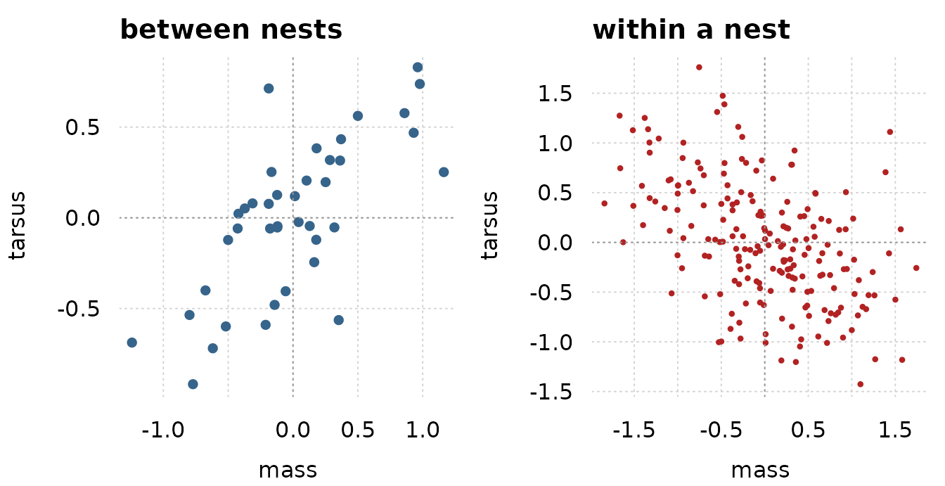
par(pp)The two clouds lean opposite ways, and that is the whole point of fitting the two correlations separately. Read the clouds for their direction and not for their strength. The nest effects are shrunk toward zero, so the left cloud looks more correlated than the number the model reports.
What this does not cover
rescor needs all gaussian or all Student-t responses. It
describes the residuals of the responses, so it cannot be combined with
a term that already describes them. An ar(),
ma(), arma(), cosy() or
unstr() term next to rescor = TRUE is refused,
and so are mixtures and censored responses. One |ID| label
must name one grouping specification: the same label over two different
grouping factors is an error, because there is no single block for it to
build. residuals() and fitted() are not the
only parts of the post-fitting surface that step back from a
rescor = TRUE fit. frm_compat("rescor") lists
the whole set, and vignette("compatibility") says why the
list is worth reading before the fit rather than after it.
10. Function-on-scalar regression
In functional data analysis the response of one subject is a whole
curve rather than a number. Function-on-scalar regression puts a
regression on such a response:
y_i(t) = b0(t) + x_i * b1(t) + e_i(t), where the
coefficients are functions of t and x_i is an
ordinary scalar covariate. This is the model of Goldsmith’s IWAFDA short
course and of refund::pffr.
frmtmb has no functional-response data structure, and does not need
one. Put the curves in long format, one row per subject and time point,
and the coefficient functions become smooths: s(t) is
b0(t) and s(t, by = x) is b1(t).
That is the same reduction mgcv uses, so mgcv is the exact
reference.
set.seed(101)
N <- 40L
tt <- seq(0, 1, length.out = 21)
x <- rbinom(N, 1, 0.5)
b0 <- function(t) 1 + 2 * sin(2 * pi * t)
b1 <- function(t) 1.5 - 12 * (t - 0.5)^2
bi <- matrix(rnorm(N * 2, 0, 0.6), N, 2)      # a per-subject curve
Y <- outer(rep(1, N), b0(tt)) + outer(x, b1(tt)) +
  bi[, 1] + outer(bi[, 2], tt - 0.5) * 2 +
  matrix(rnorm(N * length(tt), 0, 0.35), N, length(tt))
fos <- data.frame(subject = factor(rep(seq_len(N), each = length(tt))),
                  t = rep(tt, N), x = rep(x, each = length(tt)),
                  y = as.vector(t(Y)))
str(fos, give.attr = FALSE)
#> 'data.frame':    840 obs. of  4 variables:
#>  $ subject: Factor w/ 40 levels "1","2","3","4",..: 1 1 1 1 1 1 1 1 1 1 ...
#>  $ t      : num  0 0.05 0.1 0.15 0.2 0.25 0.3 0.35 0.4 0.45 ...
#>  $ x      : int  0 0 0 0 0 0 0 0 0 0 ...
#>  $ y      : num  1.15 1.34 2.52 3.07 2.8 ...
The fixed coefficient functions
ffix <- frm(bf(y ~ s(t, k = 10) + s(t, by = x, k = 10)),
            family = gaussian(), data = fos)
confint_varcorr(ffix)
#>    block       term type estimate      lwr      upr
#> 1   s(t) sd(wiggle)   sd 4.687071 2.828627 7.766536
#> 2 s(t):x sd(wiggle)   sd 2.131125 1.169335 3.883996
Each smooth contributes one variance component, and its smoothing
parameter is sigma^2 divided by that variance. Read the
coefficient functions off frm_linpred(): b0(t)
is the prediction at x = 0 and b1(t) is the
contrast between x = 1 and x = 0 at the same
t.
sg <- seq(0, 1, length.out = 9)
g0 <- data.frame(t = sg, x = 0, subject = fos$subject[1])
g1 <- data.frame(t = sg, x = 1, subject = fos$subject[1])
gfix <- mgcv::gam(y ~ s(t, k = 10) + s(t, by = x, k = 10), data = fos,
                  method = "ML")
b1_frm <- frm_linpred(ffix, newdata = g1) - frm_linpred(ffix, newdata = g0)
b1_gam <- predict(gfix, newdata = g1) - predict(gfix, newdata = g0)
out <- rbind(frmtmb = as.numeric(b1_frm), mgcv = as.numeric(b1_gam),
             truth = b1(sg))
colnames(out) <- paste0("t=", round(sg, 3))
round(out, 4)
#>          t=0 t=0.125 t=0.25 t=0.375  t=0.5 t=0.625 t=0.75 t=0.875     t=1
#> frmtmb -1.58 -0.2949 0.6985  1.3498 1.5806  1.3865 0.8644 -0.0411 -1.1534
#> mgcv   -1.58 -0.2949 0.6985  1.3498 1.5806  1.3865 0.8644 -0.0411 -1.1533
#> truth  -1.50 -0.1875 0.7500  1.3125 1.5000  1.3125 0.7500 -0.1875 -1.5000
c(max_abs_difference = max(abs(b1_frm - b1_gam)),
  frmtmb_logLik = as.numeric(logLik(ffix)),
  mgcv_ML_score = unname(-gfix$gcv.ubre),
  smoothing_par_ratio = max(abs(
    sigma(ffix)^2 / suppressWarnings(confint_varcorr(ffix))$estimate^2 /
      gfix$sp - 1)))
#>  max_abs_difference       frmtmb_logLik       mgcv_ML_score smoothing_par_ratio
#>        1.786502e-06       -9.809097e+02       -9.809097e+02        8.691598e-05
stopifnot(max(abs(b1_frm - b1_gam)) < 1e-4,
          abs(as.numeric(logLik(ffix)) + gfix$gcv.ubre) < 1e-5)
The two fitted coefficient functions agree to about 2e-6, and the
smoothing parameters to about 1e-4 relative. The middle line is the
stronger check. frmtmb reports the marginal log likelihood,
with the smooth coefficients integrated out as random effects, and that
is exactly the quantity mgcv maximizes when method = "ML"
selects the smoothing parameters. The two numbers match to 1e-8. Note
that logLik() on a gam object is not this
quantity: it is the unpenalized likelihood at the fit, so it is the
larger number and it is not comparable across the two packages.
The subject-level functional random effect
A curve per subject is a random effect that is itself a function of
t. mgcv writes it as a factor-smooth interaction,
bs = "fs", which gives every level of the factor its own
smooth with one shared set of smoothing parameters. That basis survives
frmtmb’s smooth machinery, which is mgcv::smoothCon()
followed by mgcv::smooth2random(), so the honest FoSR
spelling has it:
ffs <- frm(bf(y ~ s(t, k = 10) + s(t, by = x, k = 10) +
                s(t, subject, bs = "fs", k = 5)),
           family = gaussian(), data = fos)
confint_varcorr(ffs)
#>          block       term type  estimate        lwr       upr
#> 1         s(t) sd(wiggle)   sd 4.5736104 2.78946614 7.4988946
#> 2       s(t):x sd(wiggle)   sd 2.2368624 1.24058696 4.0332145
#> 3 s(t,subject) sd(wiggle)   sd 0.1906011 0.08490249 0.4278881
#> 4 s(t,subject) sd(wiggle)   sd 4.0785991 3.25741563 5.1068001
#> 5 s(t,subject) sd(wiggle)   sd 2.4568704 1.94615512 3.1016088
The fs term expands into three variance components,
which is how smooth2random() splits the wiggly part from
the two null-space directions of the per-subject curve. mgcv chooses
three smoothing parameters for the same term, and the fits still
agree.
gfs <- mgcv::gam(y ~ s(t, k = 10) + s(t, by = x, k = 10) +
                   s(t, subject, bs = "fs", k = 5), data = fos,
                 method = "ML")
#> Warning in gam.side(sm, X, tol = .Machine$double.eps^0.5): model has repeated
#> 1-d smooths of same variable.
b1_frm2 <- frm_linpred(ffs, newdata = g1) - frm_linpred(ffs, newdata = g0)
b1_gam2 <- predict(gfs, newdata = g1) - predict(gfs, newdata = g0)
c(max_abs_difference = max(abs(b1_frm2 - b1_gam2)),
  frmtmb_logLik = as.numeric(logLik(ffs)),
  mgcv_ML_score = unname(-gfs$gcv.ubre),
  sigma_frmtmb = sigma(ffs), sigma_mgcv = sqrt(gfs$sig2))
#> max_abs_difference      frmtmb_logLik      mgcv_ML_score       sigma_frmtmb
#>       3.059642e-06      -4.401678e+02      -4.401678e+02       3.266000e-01
#>         sigma_mgcv
#> 3.270416e-01mgcv warns that the model has repeated one-dimensional smooths of the
same variable. That is its identifiability check on s(t)
against the per-subject term, and the two are separated here by the
sum-to-zero constraint the factor-smooth basis carries. The warning is
mgcv’s, not frmtmb’s, and both packages fit the same model in spite of
it.
The per-subject curve is worth having. It takes three parameters and moves AIC by about 1000.
fre <- frm(bf(y ~ s(t, k = 10) + s(t, by = x, k = 10) + (1 + t | subject)),
           family = gaussian(), data = fos)
c(fixed_only = AIC(ffix), factor_smooth = AIC(ffs),
  random_line = AIC(fre))
#>    fixed_only factor_smooth   random_line
#>     1975.8194      900.3357      901.6500
The third fit is the cheaper alternative: a random intercept and a
random slope in t per subject, which is a straight line per
subject rather than a curve. It costs the same three parameters here and
is close behind. Use it when the per-subject departures are near linear,
and use bs = "fs" when they are not.
xg <- data.frame(t = seq(0, 1, length.out = 100), x = 0,
                 # an UNSEEN subject: mgcv's fs basis returns a zero row
                 # for a level it does not know, so the per-subject curve
                 # contributes nothing and this IS the population
                 # coefficient function. re_formula = NA would not do it:
                 # it keeps every smooth, as brms does, and removes the
                 # (x | g) group-level terms alone
                 subject = factor("population",
                                  levels = c(levels(fos$subject),
                                             "population")))
xg1 <- transform(xg, x = 1)
f0 <- as.numeric(frm_linpred(ffs, newdata = xg, allow_new_levels = TRUE))
f1 <- as.numeric(frm_linpred(ffs, newdata = xg1,
                             allow_new_levels = TRUE)) - f0
tinyplot::tinyplot(x = xg$t, y = f0, type = "l", col = "steelblue4",
                   lwd = 2, theme = "clean2", xlab = "t",
                   ylab = "coefficient function",
                   ylim = range(c(f0, f1, b0(xg$t), b1(xg$t))))
tinyplot::plt_add(x = xg$t, y = f1, type = "l", col = "firebrick", lwd = 2)
lines(xg$t, b0(xg$t), lty = 2, col = "gray40")
lines(xg$t, b1(xg$t), lty = 2, col = "gray40")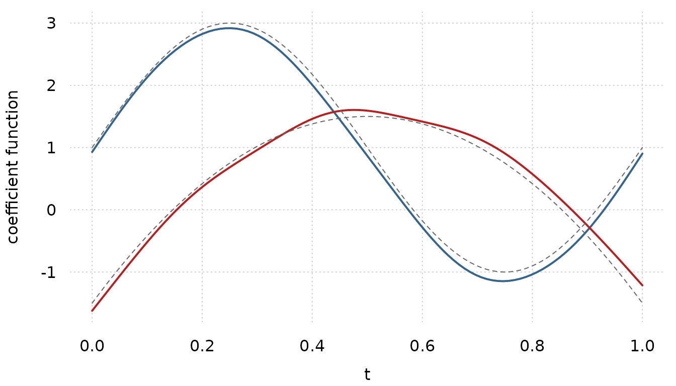
Scalar-on-function regression
The mirror model has a scalar response and a functional predictor:
y_i = a + integral of b(s) X_i(s) ds. Approximate the
integral by a quadrature sum and it becomes a smooth of s
weighted by the observations, which mgcv spells
s(S, by = L) where S and L are
matrix columns of the data frame: S holds
the grid and L holds the quadrature weight times the
observed function.
Matrix columns are accepted in a frmtmb design matrix, so this spelling works unchanged.
set.seed(202)
n <- 150L; nS <- 30L
S <- seq(0, 1, length.out = nS)
beta_f <- function(s) 2 * sin(2 * pi * s)
Xf <- t(replicate(n, cumsum(rnorm(nS, 0, 0.4)) + rnorm(nS, 0, 0.2)))
sof <- data.frame(y = 1 + as.vector((Xf / nS) %*% beta_f(S)) +
                    rnorm(n, 0, 0.4))
sof$Smat <- matrix(S, n, nS, byrow = TRUE)      # the grid, one row per case
sof$LX <- Xf / nS                               # weight times observation
vapply(sof, function(z) sprintf("%s, %d column(s)", class(z)[1], NCOL(z)), "")
#>                      y                   Smat                     LX
#> "numeric, 1 column(s)" "matrix, 30 column(s)" "matrix, 30 column(s)"
fsof <- frm(bf(y ~ s(Smat, by = LX, k = 12)), family = gaussian(),
            data = sof)
gsof <- mgcv::gam(y ~ s(Smat, by = LX, k = 12), data = sof, method = "ML")
c(frmtmb_sigma = sigma(fsof), mgcv_sigma = sqrt(gsof$sig2),
  max_abs_fitted_difference =
    max(abs(fitted(fsof)[, "Estimate"] - as.numeric(fitted(gsof)))))
#>              frmtmb_sigma                mgcv_sigma max_abs_fitted_difference
#>              3.879616e-01              3.898877e-01              7.714926e-08
Recover b(s) by predicting at a synthetic case whose
weight vector is one in a single grid cell and zero elsewhere. The
linear functional term then reduces to b(s) at that
cell.
sgrid <- seq(0, 1, length.out = 9)
nd <- sof[rep(1, length(sgrid)), "y", drop = FALSE]
nd$Smat <- matrix(sgrid, length(sgrid), nS)
nd$LX <- cbind(1, matrix(0, length(sgrid), nS - 1))
out <- rbind(frmtmb = as.numeric(frm_linpred(fsof, newdata = nd)),
             mgcv = as.numeric(predict(gsof, newdata = nd)),
             truth_plus_intercept = beta_f(sgrid) + 1)
colnames(out) <- paste0("s=", round(sgrid, 3))
round(out, 4)
#>                         s=0 s=0.125 s=0.25 s=0.375  s=0.5 s=0.625  s=0.75
#> frmtmb               2.6383  3.0372 2.8772  2.0599 0.7948 -0.4055 -0.9728
#> mgcv                 2.6383  3.0372 2.8772  2.0599 0.7948 -0.4055 -0.9728
#> truth_plus_intercept 1.0000  2.4142 3.0000  2.4142 1.0000 -0.4142 -1.0000
#>                      s=0.875   s=1
#> frmtmb               -0.3896 1.064
#> mgcv                 -0.3896 1.064
#> truth_plus_intercept -0.4142 1.000
stopifnot(max(abs(fitted(fsof)[, "Estimate"] -
                    as.numeric(fitted(gsof)))) < 1e-5)
The two coefficient functions are the same to four decimal places,
and the fitted values to 1e-7. Both depart from the truth at
s = 0, which is the usual endpoint behavior of a linear
functional term: the quadrature gives the first grid cell one weight out
of thirty, so the data say little about the curve there.
What this does not cover. There is no functional-response object, so
the grid must be in long format and an irregular grid is simply an
irregular t column. There is no penalty that couples
b0(t) and b1(t). And
conditional_effects() will not draw a term built on matrix
columns:
conditional_effects(fsof)
#> Error:
#> ! conditional_effects() has nothing to draw for dpar 'mu': the only predictor(s) of that parameter are the matrix column(s) `Smat` (carried by s(Smat):LX), which the display excludes. A matrix column is a whole function per row, so it has neither a one-dimensional axis to vary along nor a single value to hold the other predictors at. Draw the coefficient function with predict(newdata = ) over a grid you build yourself: one row per grid point, the matrix column holding the grid, and the weight column an indicator of the point
The refusal names the matrix columns itself and points at the way
out. Draw the coefficient function from frm_linpred() as
above.
11. A custom family with a bounded parameter
A family here is an R function that returns a log density, and the
tape differentiates it. vignette("frmtmb") writes the
smallest one there is: a Poisson, one distributional parameter, one link
named by string. This section writes the next one up. Three
distributional parameters, a link that no name covers, and a support
that depends on a parameter the model estimates.
The example is the shifted lognormal, which brms spells
shifted_lognormal(): a lognormal density displaced by a
shift, read in response-time work as the time the process spent doing
something other than what the lognormal describes. frmtmb has that
family built in, and that is the point of choosing it. The built-in is
an exact reference for the custom version, so the section ends with a
check that holds to machine precision rather than an appeal to
plausibility.
The density
The density of y = shift + Lognormal(mu, sigma) follows
from the change of variables z = log(y - shift), whose
Jacobian contributes the -z term:
The link that no name covers
The density is defined only for y > shift, so the
support moves with a parameter. The built-in family gives
shift a log link and lets the optimizer discover the
boundary: a step past min(y) makes the objective
NaN, which nlminb treats as a rejected step. That works,
and it depends on the optimizer’s response to a NaN.
The alternative is to make the constraint structural. Give the shift
a logit scaled onto (0, U), with U fixed when
the family is built, and no finite linear predictor can violate the
support. A link is a list of name, linkfun,
linkinv and mu_eta, and every place that takes
a link name takes such a list instead.
shifted_ln <- function(max_shift) {
  force(max_shift)
  shift_link <- list(
    name = "scaled_logit",
    linkfun = function(mu) log(mu / (max_shift - mu)),
    linkinv = function(eta) max_shift / (1 + exp(-eta)),
    mu_eta = function(eta) {
      p <- 1 / (1 + exp(-eta)); max_shift * p * (1 - p)
    })
  custom_family(
    "shifted_ln",
    dpars = c("mu", "sigma", "shift"),
    links = list(mu = "identity", sigma = "log", shift = shift_link),
    lpdf = function(y, dpars, aterms) {
      sln_lpdf(y, dpars$mu, dpars$sigma, dpars$shift)
    },
    init_dpars = list(
      mu = function(y, aterms) mean(log(y - min(y) / 2)),
      sigma = function(y, aterms) stats::sd(log(y - min(y) / 2)),
      shift = function(y, aterms) min(y) / 2),
    type = "continuous")
}
init_dpars reads the data and returns a starting value
per parameter on the RESPONSE scale; the link puts it on the
linear-predictor scale. A bounded link needs that start to be inside the
bound, which is why min(y) / 2 rather than
min(y).
The one arithmetic caveat is the same one every bounded link has.
Past a linear predictor near 37 the logit saturates in double precision
and the shift rounds to U exactly. The density keeps the
optimizer away from that corner, because the log likelihood falls off
long before the link saturates.
Check it before fitting it
check_custom_family() evaluates the density on a tape,
compares its gradient against a finite difference, and re-tapes to catch
the mistakes that make a family work once and fail on the second call.
Because the density is plain arithmetic, the same function also checks
against a closed form: dlnorm() at the shifted
response.
set.seed(12)
probe <- 0.3 + rlnorm(50, -0.4, 0.35)
check_custom_family(shifted_ln(max_shift = 0.3), y = probe,
                    dpars = list(mu = rep(-0.4, 50),
                                 sigma = rep(0.35, 50),
                                 shift = rep(0.15, 50)))
sln_grid <- expand.grid(y = c(0.35, 0.6, 1.2, 3), mu = c(-1, 0, 1),
                        sigma = c(0.2, 0.8), shift = c(0.05, 0.3))
with(sln_grid, {
  ref <- dlnorm(y - shift, mu, sigma, log = TRUE)
  c(cases = length(ref),
    max_relative_error = max(abs(sln_lpdf(y, mu, sigma, shift) - ref) /
                               abs(ref)))
})
#>              cases max_relative_error
#>       4.800000e+01       7.012572e-16
Fitting
set.seed(11)
sln_d <- data.frame(x = rnorm(400))
sln_d$rt <- 0.25 + rlnorm(400, -0.4 + 0.3 * sln_d$x, 0.35)
fsl <- frm(bf(rt ~ x), family = shifted_ln(max_shift = min(sln_d$rt)),
           data = sln_d)
e <- unlist(fixef_by_dpar(fsl))
shift_hat <- min(sln_d$rt) / (1 + exp(-e[["shift.(Intercept)"]]))
out <- rbind(
  estimated = c(e[["mu.(Intercept)"]], e[["mu.x"]],
                exp(e[["sigma.(Intercept)"]]), shift_hat),
  simulated = c(-0.4, 0.3, 0.35, 0.25))
colnames(out) <- c("mu_intercept", "mu_slope", "sigma", "shift")
round(out, 3)
#>           mu_intercept mu_slope sigma shift
#> estimated       -0.425    0.303 0.371 0.281
#> simulated       -0.400    0.300 0.350 0.250
The shift is the parameter the data speak about least. Only the smallest response times carry information about it, so its standard error is wide and its point estimate sits above the generating value here. Read it with the interval rather than on its own:
Cross-check against the built-in family
The built-in shifted_lognormal() is the same likelihood
under a different link for the shift. A reparameterization moves the
optimizer path, not the optimum, so both fits should reach the same
maximum and the same shift on the response scale.
fbi <- frm(bf(rt ~ x), family = shifted_lognormal(), data = sln_d)
eb <- unlist(fixef_by_dpar(fbi))
c(custom = as.numeric(logLik(fsl)), builtin = as.numeric(logLik(fbi)),
  loglik_difference = as.numeric(logLik(fsl)) - as.numeric(logLik(fbi)),
  shift_difference = shift_hat - exp(eb[["ndt.(Intercept)"]]))
#>            custom           builtin loglik_difference  shift_difference
#>      1.478009e+00      1.478009e+00     -8.881784e-15      2.230538e-09
stopifnot(
  abs(as.numeric(logLik(fsl)) - as.numeric(logLik(fbi))) < 1e-6,
  abs(shift_hat - exp(eb[["ndt.(Intercept)"]])) < 1e-4,
  with(sln_grid, max(abs(sln_lpdf(y, mu, sigma, shift) -
                           dlnorm(y - shift, mu, sigma, log = TRUE)))) <
    1e-12)
That equality is the check to write for any custom family that shadows something already implemented, in this package or another one. It costs one extra fit and it tests the whole path: the density, the links, the starts and the optimizer.
The harder cases, and where they went
A drift-diffusion model sat in this slot until frmtmb.eam existed: a
first-passage density written as a series, a boundary indicator arriving
through vint(), and a non-decision time bounded exactly as
the shift is above. That family is a package now, and the package does
the density better than a case study did.
vignette("ddm", package = "frmtmb.eam") is the worked
model, and frmtmb.eam::wiener() is the family.
Two lessons live there rather than here:
- An integer covariate reaching the density through
vint(), which arrives as theatermsargument of thelpdf.?custom_familyhas a worked example of that, and the ddm vignette explains why the decision indicator has to travel that way. - What to do when the density is a series whose term count would have to depend on a parameter. The tape cannot branch on a parameter, so the choice is between one fixed truncation, which fails outside the range it covers, and evaluating both series and blending them. The ddm vignette measures both.
12. Circular regression
Wind direction, the phase of a circadian rhythm and the bearing of a
migrating bird are angles. Their arithmetic wraps, so a linear model of
the number is wrong at the wrap point: 359 degrees and 1 degree are two
degrees apart, not 358. von_mises() is the natural
exponential family on the circle, with a mean direction mu
and a concentration kappa (Fisher 1993; Mardia and Jupp
2000).
The example is the sea breeze: wind direction at a coastal station
rotates through the day, and the breeze is both steadier and stronger in
the afternoon. Both facts are in the model, because kappa
takes a formula of its own.
# exact rejection sampling from a von Mises, uniform proposal
rvon_mises <- function(n, mu, kappa) {
  mu <- rep_len(mu, n); kappa <- rep_len(kappa, n)
  th <- numeric(n); todo <- seq_len(n)
  while (length(todo)) {
    z <- runif(length(todo), -pi, pi)
    ok <- runif(length(todo)) < exp(kappa[todo] * (cos(z) - 1))
    th[todo[ok]] <- z[ok]
    todo <- todo[!ok]
  }
  ((th + mu + pi) %% (2 * pi)) - pi
}
set.seed(77)
nw <- 600
hour <- runif(nw, 0, 24)
mu_true <- 2 * atan(0.6 * sin(2 * pi * hour / 24))
kappa_true <- exp(0.7 + 0.8 * cos(2 * pi * (hour - 15) / 24))
wind <- data.frame(hour = hour,
                   angle = rvon_mises(nw, mu_true, kappa_true))
bs = "cc" is mgcv’s cyclic cubic spline, whose value and
first two derivatives match at the ends of the range. That is the right
basis for a covariate that is itself periodic, and it saves the model
from predicting a jump at midnight.
fvm <- frm(bf(angle ~ s(hour, bs = "cc", k = 8),
              kappa ~ s(hour, bs = "cc", k = 8)),
           family = von_mises(), data = wind)
nd <- data.frame(hour = c(0, 6, 12, 18))
out <- rbind(
  mu_estimated = as.numeric(frm_linpred(fvm, newdata = nd, type = "response")),
  mu_simulated = 2 * atan(0.6 * sin(2 * pi * nd$hour / 24)),
  kappa_estimated = as.numeric(frm_linpred(fvm, newdata = nd, dpar = "kappa",
                                       type = "response")),
  kappa_simulated = exp(0.7 + 0.8 * cos(2 * pi * (nd$hour - 15) / 24)))
colnames(out) <- paste0("hour ", nd$hour)
round(out, 3)
#>                 hour 0 hour 6 hour 12 hour 18
#> mu_estimated     0.101  1.083   0.097  -1.118
#> mu_simulated     0.000  1.081   0.000  -1.081
#> kappa_estimated  1.341  1.060   3.924   3.782
#> kappa_simulated  1.144  1.144   3.546   3.546
The mean direction is reported in radians on (-pi, pi).
The link is tan_half, mu = 2 * atan(eta),
which maps the whole line onto that interval, so the linear predictor is
not itself an angle.
Cross-check against the closed-form circular MLE
For an intercept-only model the maximum likelihood estimates are
known in closed form. The mean direction is the direction of the mean
resultant vector, and the concentration solves
A1(kappa) = I1(kappa) / I0(kappa) = Rbar, where
Rbar is the length of that vector. Neither expression uses
any part of frmtmb.
set.seed(78)
w0 <- data.frame(angle = rvon_mises(500, 0.8, 2.2))
f0 <- frm(bf(angle ~ 1), family = von_mises(), data = w0)
Rbar <- sqrt(mean(sin(w0$angle))^2 + mean(cos(w0$angle))^2)
out <- rbind(
  frmtmb = c(as.numeric(frm_linpred(f0, newdata = w0[1, , drop = FALSE],
                                type = "response")),
             exp(unlist(fixef_by_dpar(f0)$kappa))),
  closed_form = c(atan2(mean(sin(w0$angle)), mean(cos(w0$angle))),
                  uniroot(function(k) besselI(k, 1) / besselI(k, 0) - Rbar,
                          c(1e-8, 500), tol = 1e-12)$root),
  simulated = c(0.8, 2.2))
colnames(out) <- c("mean_direction", "kappa")
round(out, 6)
#>             mean_direction    kappa
#> frmtmb            0.823811 2.289763
#> closed_form       0.823811 2.289763
#> simulated         0.800000 2.200000
stopifnot(
  abs(as.numeric(frm_linpred(f0, newdata = w0[1, , drop = FALSE],
                         type = "response")) -
        atan2(mean(sin(w0$angle)), mean(cos(w0$angle)))) < 1e-6,
  abs(exp(unlist(fixef_by_dpar(f0)$kappa)) -
        uniroot(function(k) besselI(k, 1) / besselI(k, 0) - Rbar,
                c(1e-8, 500), tol = 1e-12)$root) < 1e-5)
Both estimates match the closed form to six decimal places.
circular::mle.vonmises() gives the same mean direction and
a concentration that differs in the fourth decimal, because it applies a
small-sample bias correction to kappa by default.
m <- circular::mle.vonmises(circular::circular(w0$angle))
c(circular_mu = as.numeric(m$mu), circular_kappa = as.numeric(m$kappa))
#>    circular_mu circular_kappa
#>      0.8238112      2.2829061
The daily cycle is easier to see on the circle than in a table.
hg <- data.frame(hour = seq(0, 24, length.out = 200))
mu_g <- as.numeric(frm_linpred(fvm, newdata = hg, type = "response"))
kp_g <- as.numeric(frm_linpred(fvm, newdata = hg, dpar = "kappa",
                           type = "response"))
op <- par(mfrow = c(2, 1), mar = c(4, 4, 1, 1))
tinyplot::tinyplot(angle ~ hour, data = wind, type = "p", pch = 16,
                   cex = 0.5, col = "gray55", theme = "clean2",
                   xlab = "", ylab = "direction (rad)")
lines(hg$hour, mu_g, col = "steelblue4", lwd = 2)
lines(hg$hour, 2 * atan(0.6 * sin(2 * pi * hg$hour / 24)), lty = 2,
      col = "gray30")
tinyplot::tinyplot(x = hg$hour, y = kp_g, type = "l", col = "firebrick",
                   lwd = 2, theme = "clean2", xlab = "hour of day",
                   ylab = "kappa", ylim = c(0, max(kp_g) * 1.1))
lines(hg$hour, exp(0.7 + 0.8 * cos(2 * pi * (hg$hour - 15) / 24)),
      lty = 2, col = "gray30")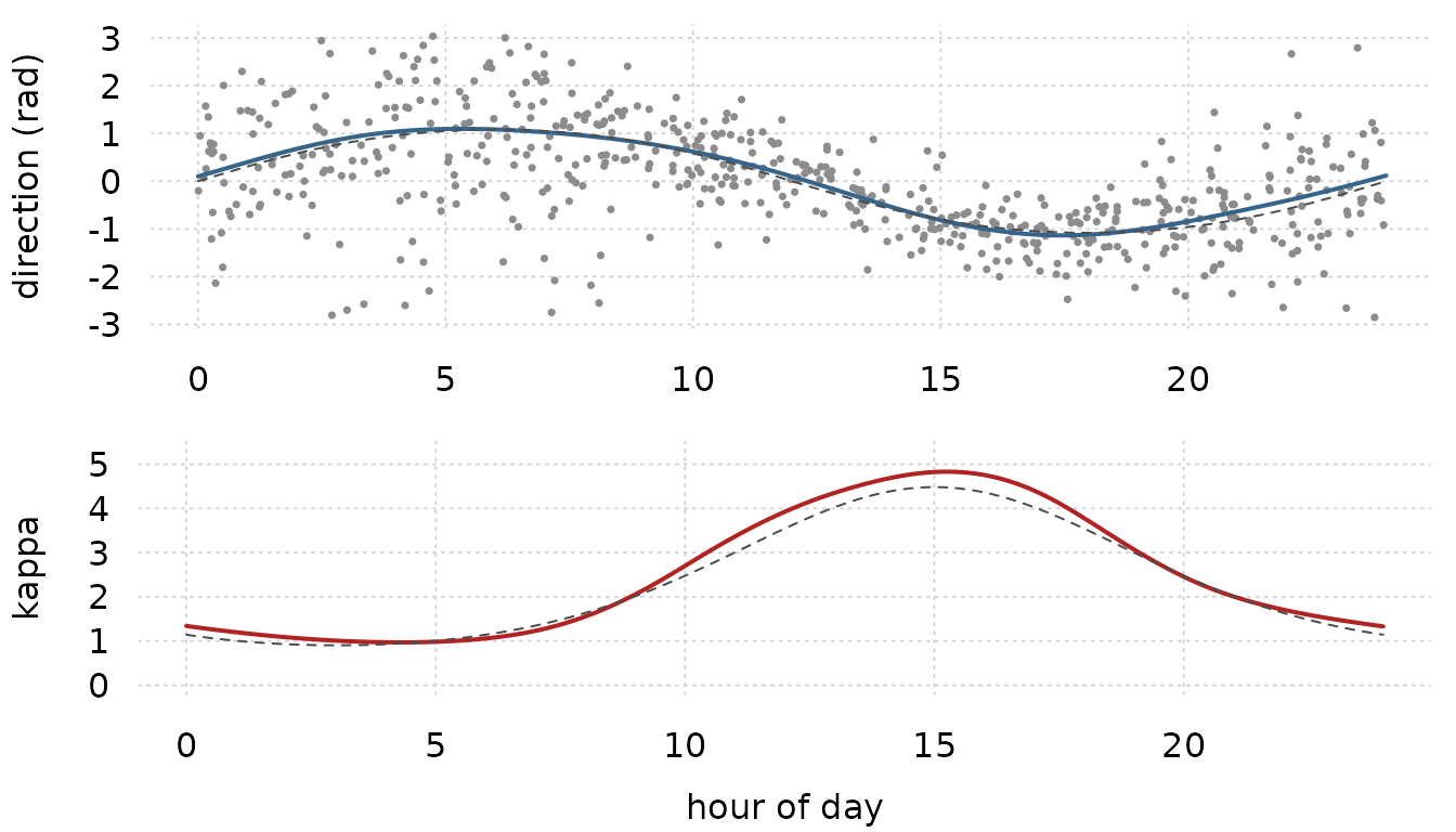
par(op)The points crowd around the blue line in the afternoon and spread out before dawn, which is the red curve read off the data.
What this does not cover. von_mises() is the only
circular family here: there is no wrapped normal, wrapped Cauchy or
projected normal. The response must be in radians on
(-pi, pi]; a response in degrees or on
[0, 2 pi) fits a different model and is refused. The
predictor is a number rather than an angle, so this is circular-linear
regression, not circular-circular regression; a periodic covariate
enters through a cyclic basis as above. And the tan_half
link puts a mean direction near the ends of the range at the ends of the
link’s range too, so a phenomenon centered near pi should
be rotated to the middle of the interval before fitting.
13. A warped population growth curve
The models above all add a smooth to a linear predictor. This one does not: it estimates ONE population curve and lets each child see it shifted along its own time axis, which is a semiparametric nonlinear mixed-effects model (SNMM) in the sense of Ke and Wang (2001). The version fitted here is D’Alessandro, Thoresen and Sorensen (2026, arXiv:2603.11728), who apply it to infant height in the first two years of life:
with
and
.
f is the population growth curve,
moves a child up or down,
moves it earlier or later along the age axis, and
says how much of that timing shift a week of gestational age buys.
Nothing in s(x) can express this. A penalized smooth’s
basis is evaluated at a COLUMN, so the frame can build Z
once and the objective adds Z b to a predictor. Here the
spline’s argument contains b_{2i}, which is a parameter, so
there is no fixed Z to build: the basis has to be evaluated
on the tape, at a point the fit moves. ps() is the term for
that. It is admitted only inside a nonlinear body, it evaluates to the
spline’s VALUE rather than adding itself to anything, and it carries the
same mixed-model split s() does: the null space of the
second-difference penalty joins the fixed coefficients and the range
space becomes one random-effect block whose single variance is the
inverse smoothing parameter.
The data are brokenstick::smocc_200: 1942 height
measurements on 200 Dutch children, 6 to 12 each. Age goes in as weeks
so that
is a shift in weeks per week of gestation, and gestational age is
centered at 40.
raw <- brokenstick::smocc_200
smocc <- data.frame(
  id  = factor(raw$id),
  age = 52.1775 * raw$age,          # years to weeks
  sex = as.numeric(raw$sex == "male"),
  ga  = raw$ga - 40,                # weeks from term
  hgt = raw$hgt)
smocc <- smocc[!is.na(smocc$hgt), ]
smocc$id <- droplevels(smocc$id)
c(rows = nrow(smocc), children = nlevels(smocc$id))
#>     rows children
#>     1906      200
fit_smocc <- frm(
  bf(hgt ~ int + exp(amp) * ps(age + shift, k = 15, pad = 0.25),
     int   ~ sex + (1 | id),
     amp   ~ 0 + sex,
     shift ~ 0 + ga + (1 | id),
     nl = TRUE),
  data = smocc, family = gaussian(),
  start = list(beta = c(68, 2, 0, 1, 0)))
fixef_by_dpar(fit_smocc)[c("int", "amp", "shift")]
#> $int
#> (Intercept)         sex
#>   68.754333    1.805782
#>
#> $amp
#>          sex
#> 0.0002123576
#>
#> $shift
#>       ga
#> 1.050019
VarCorr(fit_smocc)
#> $id
#> $id$sd
#>                 Estimate Est.Error     Q2.5    Q97.5
#> int_Intercept   2.868475 0.1560077 2.562706 3.174245
#> shift_Intercept 3.324130 0.2122613 2.908105 3.740154
#>
#>
#> $residual__
#> $residual__$sd
#>  Estimate  Est.Error     Q2.5    Q97.5
#>  1.056744 0.01987038 1.017798 1.095689
k = 15 is the paper’s cubic basis with 11 interior
knots. pad = 0.25 widens the range the knots are placed on
before they are frozen: the spline is evaluated at
age + shift, the fitted shift SD is over three weeks, and
the basis is exactly zero outside its knot span, so the padding has to
cover where the fit will actually look. frm() reports at
the end how many rows fell outside it, and frm_linpred()
reports it again for a grid that leaves the span.
The knot RULE is not the paper’s, and this section is not a
reimplementation of it. The paper’s section 2.3.1 rescales the spline
argument to [0, 1] between bounds that move with the
current variance estimates, so its knots follow the fit;
ps() freezes knots on a padded data range, because moving
knots make the penalty matrix and its eigendecomposition functions of
the parameters and because a basis rebuilt between fitting and
prediction is a different basis. The two are related constructions that
agree on this application. See ?ps.
The estimates against the paper’s Table 1:
fx <- fixef_by_dpar(fit_smocc)
vc <- VarCorr(fit_smocc)
got <- c(beta0 = fx$int[["(Intercept)"]], beta1 = fx$int[["sex"]],
         beta2 = fx$amp[["sex"]],         beta3 = fx$shift[["ga"]],
         sd_b1 = vc$id$sd["int_Intercept", "Estimate"],
         sd_b2 = vc$id$sd["shift_Intercept", "Estimate"],
         sigma = exp(fx$sigma[["(Intercept)"]]))
paper <- c(beta0 = 68.2, beta1 = 1.80, beta2 = 0.00, beta3 = 1.00,
           sd_b1 = 2.86, sd_b2 = 3.28, sigma = 1.05)
round(cbind(frmtmb = got, paper = paper, difference = got - paper), 3)
#>       frmtmb paper difference
#> beta0 68.754 68.20      0.554
#> beta1  1.806  1.80      0.006
#> beta2  0.000  0.00      0.000
#> beta3  1.050  1.00      0.050
#> sd_b1  2.868  2.86      0.008
#> sd_b2  3.324  3.28      0.044
#> sigma  1.057  1.05      0.007
Six of the seven agree to the published precision. The intercept is
0.55 cm higher, and that is an identifiability convention rather than a
disagreement. ps() constrains the spline’s COEFFICIENTS to
sum to zero. The paper says only that it applies “a sum-to-zero
constraint to ensure identifiability of an intercept term” and does not
say on what, so the right thing to do is measure rather than attribute:
re-centering the curve to its own fitted values moves the intercept onto
the published one.
pt <- fit_smocc$frame$linpreds[["hgt.mu"]]$ps_terms[[1]]
bk <- fit_smocc$frame$re_blocks[[pt$block_id]]
p <- fit_smocc$estimates
bn <- names(fit_smocc$frame$par_template$beta)
gam <- as.vector(pt$U0 %*% p$beta[pt$beta_idx] + pt$Us %*% p$b[bk$b_idx])
arg <- smocc$age + p$beta[match("shift_ga", bn)] * smocc$ga +
  p$b[fit_smocc$frame$re_blocks[[2]]$b_idx][as.integer(smocc$id)]
curve_at_data <- as.vector(
  splines::splineDesign(pt$knots, arg, ord = pt$ord,
                        outer.ok = TRUE) %*% gam)
c(beta0 = p$beta[match("int_(Intercept)", bn)],
  recentred = p$beta[match("int_(Intercept)", bn)] + mean(curve_at_data),
  paper = 68.2)
#>     beta0.int_(Intercept) recentred.int_(Intercept)                     paper
#>                  68.75433                  68.19824                  68.20000
Whatever the paper’s constraint was, the two intercepts describe the same fitted surface to 0.002 cm once the curve is centered the same way. Nothing that depends on the curve’s SHAPE moves with the convention at all.
The likelihood is checked against the paper’s equations written out
in plain R, with the basis taken from
splines::splineDesign() rather than from the branch-free
construction the objective tapes:
lp <- fit_smocc$frame$linpreds[["hgt.mu"]]
pt <- lp$ps_terms[[1]]
bk <- fit_smocc$frame$re_blocks[[pt$block_id]]
bn <- names(fit_smocc$frame$par_template$beta)
p  <- fit_smocc$estimates

gamma <- as.vector(pt$U0 %*% p$beta[pt$beta_idx] + pt$Us %*% p$b[bk$b_idx])
arg <- smocc$age + p$beta[match("shift_ga", bn)] * smocc$ga +
  p$b[fit_smocc$frame$re_blocks[[2]]$b_idx][as.integer(smocc$id)]
f_hat <- as.vector(splines::splineDesign(pt$knots, arg, ord = pt$ord,
                                         outer.ok = TRUE) %*% gamma)
mu <- p$beta[match("int_(Intercept)", bn)] +
  p$beta[match("int_sex", bn)] * smocc$sex +
  p$b[fit_smocc$frame$re_blocks[[1]]$b_idx][as.integer(smocc$id)] +
  exp(p$beta[match("amp_sex", bn)] * smocc$sex) * f_hat

blk <- function(i) fit_smocc$frame$re_blocks[[i]]
ref <- sum(dnorm(smocc$hgt, mu, exp(p$betad[1]), log = TRUE)) +
  sum(dnorm(p$b[blk(1)$b_idx], 0, exp(p$theta[blk(1)$theta_idx]),
            log = TRUE)) +
  sum(dnorm(p$b[blk(2)$b_idx], 0, exp(p$theta[blk(2)$theta_idx]),
            log = TRUE)) +
  sum(dnorm(p$b[bk$b_idx], 0, exp(p$theta[bk$theta_idx]), log = TRUE))
joint <- -frmtmb:::build_objective(fit_smocc$frame)(p)
c(frmtmb = joint, reference = ref, difference = joint - ref)
#>        frmtmb     reference    difference
#> -3.653385e+03 -3.653385e+03  6.548362e-11
stopifnot(abs(joint - ref) < 1e-8)
The curve, with a band
frm_linpred(se.fit = TRUE) refuses a nonlinear
predictor, and it is right to: the map from coefficients to
eta is not a design matrix there, it is a Jacobian.
frm_lp_basis() is the route. It tapes the body against
every coefficient the body reaches through, including the
ps() block’s own, and returns that Jacobian with the joint
covariance at exactly the rows its columns sit at.
grid <- data.frame(age = seq(0, 130, length.out = 120), sex = 0, ga = 0,
                   id = factor(levels(smocc$id)[1], levels(smocc$id)))
lb <- frm_lp_basis(fit_smocc, newdata = grid, re_formula = NA)
se <- sqrt(pmax(rowSums((lb$A %*% lb$V) * lb$A), 0))
band <- data.frame(age = grid$age, fit = lb$eta,
                   lo = lb$eta - 1.96 * se, hi = lb$eta + 1.96 * se)
head(round(band, 3), 3)
#>     age    fit     lo     hi
#> 1 0.000 49.992 49.221 50.762
#> 2 1.092 50.928 50.167 51.690
#> 3 2.185 51.850 51.097 52.603
The whole grid’s covariance, A V A', is what a
SIMULTANEOUS band needs. frm_curve() builds one from the
same two objects, and it refused a nonlinear body until this seam
existed. The band here is pointwise, to show the two objects themselves;
frm_curve() on the same grid gives the simultaneous
band.
tinyplot::tinyplot(hgt ~ age, data = smocc[smocc$id %in%
                     levels(smocc$id)[1:40], ],
                   type = "p", col = "grey70", cex = 0.4,
                   xlab = "age (weeks)", ylab = "height (cm)",
                   main = "SMOCC: population growth curve")
tinyplot::tinyplot_add(hi ~ age, data = band, type = "l", lty = 2)
tinyplot::tinyplot_add(lo ~ age, data = band, type = "l", lty = 2)
tinyplot::tinyplot_add(fit ~ age, data = band, type = "l", lwd = 2)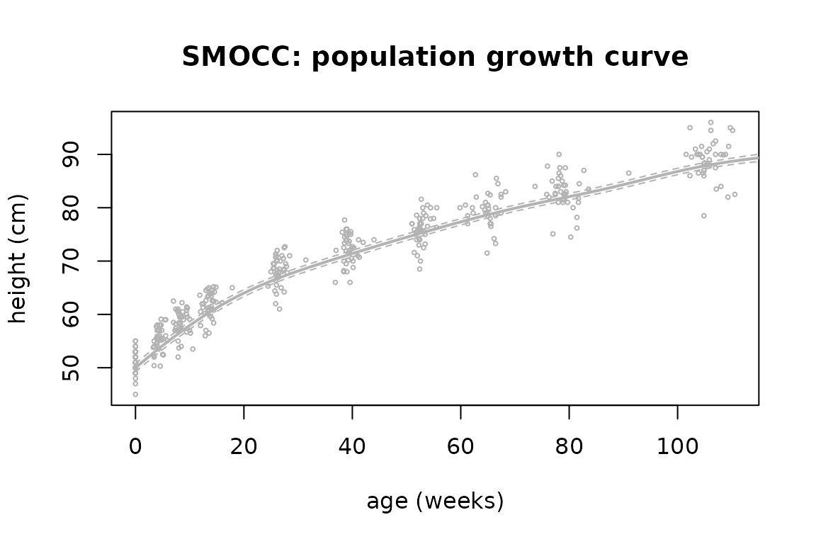
What a ps() block refuses
REML = TRUE, quadrature = TRUE,
frmtmb_control(profile = TRUE) and multivariate models are
refused by name. The first three integrate out something the block has
already put inside the Laplace approximation; the fourth is untested
rather than known to be wrong, and is refused for that reason. The
importance correction refuses every nonlinear predictor already, so a
ps() block inside one is refused by that guard rather than
by a new one.
try(frm(bf(hgt ~ int + ps(age, k = 8), int ~ 1, nl = TRUE),
        data = smocc[1:200, ], family = gaussian(), REML = TRUE))
#> Error : REML = TRUE cannot be combined with ps(age, k = 8): REML integrates the fixed coefficients out, and this term puts its own null space among them inside a body that is nonlinear in it
The basis itself is a divided difference of truncated powers written
branch free, because RTMB refuses pmax() on an AD type and
exports no CondExp, so the recursive Cox-de Boor form is
unavailable. It agrees with splines::splineDesign() to
3.1e-13 absolute at k = 12 and 1.8e-11 at
k = 40, and the error grows like
k^(degree - 1) because a divided difference cancels terms
of order (range / spacing)^degree. k above 50
is refused for that reason. See ?ps.
Where the checks live
Every cross-check on this page runs when the page is built, and the
stopifnot() calls fail the build if a number moves. The
strongest of them are also pinned in
tests/testthat/test-case-studies.R, so they run in the test
suite as well. Section 11 states the general rule: a custom family that
shadows an implemented one should be checked against it, because that
comparison exercises the density, the links, the starts and the
optimizer in one number.
Several points of friction showed up while writing these case studies, and each one is handled above:
- A
gr(cov = )block with one row per level triggers the observation-level random effect warning, although the covariance matrix identifies the two variances. Usefrmtmb_control(check_olre = "ignore"). - A multi-trait model with a known covariance can use the long format
of section 1 or
mvbf()with the|ID|identifier over the samegr(cov = )term; the two spellings are the same joint density. One|ID|label must name one grouping specification, and the matrix must resolve identically in every formula. -
logLik()means different things in frmtmb and in mgcv. frmtmb reports the marginal likelihood with the smooth coefficients integrated out, which is what mgcv maximizes undermethod = "ML"and reports as-gam$gcv.ubre.logLik.gamis the unpenalized likelihood at the fit and is the wrong number to compare against. Section 10 compares the right pair. -
re_formula = NAdoes NOT drop anfsfactor-smooth. It removes the(x | g)group-level terms and keeps every smooth, which is brms’s rule. To read the population coefficient function off such a model, predict at an UNSEEN level of the grouping factor withallow_new_levels = TRUE: mgcv’sfsbasis returns a zero row for a level it does not know, so the per-subject curve contributes nothing. Section 10 draws its figure that way. The grouping column is needed innewdataat everyre_formula. - A custom family may pass a link OBJECT rather than a link name,
which is how section 11 bounds a shift parameter by the data. The object
needs
name,linkfun,linkinvandmu_eta. -
residuals()andfitted()refuse a multivariate fit.frm_linpred()takesresp, so a fitted value for one response is one call and a residual is a subtraction. Section 9 draws its figure that way, and reads the other level of the same model out ofranef(). -
frm_linpred(se.fit = TRUE)refuses a nonlinear predictor, and aps()curve is one.frm_lp_basis()is the route: it returnsd eta / d coefas a Jacobian, taped rather than perturbed, together with the joint covariance at the rows its columns sit at. Section 13 draws its band that way. - A
ps()basis is FROZEN on the padded range of its argument at data time, with every nonlinear parameter at zero, and it is exactly zero outside that span.pad =is what covers the distance the fit then moves; a fit reports how many rows it left behind.
Some models on this page are refused by parts of the post-fitting
surface, and the refusals are deliberate. A term built on matrix columns
is excluded from conditional_effects(), because a matrix
covariate has no single value to hold the other predictors at. A family
whose likelihood does not factorize over the rows refuses more than
that.
Two subjects that were case studies here have packages of their own now, and each one carries a worked page written to this standard. Read them as the next two studies in the tour.
-
vignette("latent", package = "frmtmb.latent")fits a hidden Markov model to an animal track, cross-checks it against hmmTMB and depmixS4, and lists what a likelihood that does not factorize over the rows refuses. -
vignette("ddm", package = "frmtmb.eam")fits the drift-diffusion first-passage density of section 11, and measures the two ways of truncating its series.
The identity-refit check of section 1 belongs in any model that reads
a matrix from data2. It is the one test that a structured
covariance cannot pass by accident.