frmtmb fits regression models written in the brms formula grammar by maximum likelihood, with the Laplace approximation for random effects. The backend is RTMB: the model formula compiles to an R objective function that is differentiated on the TMB AD tape. There is no MCMC and no compilation at run time.
A mixed model
data(sleepstudy, package = "lme4")

fit <- frm(bf(Reaction ~ Days + (Days | Subject)), family = gaussian(),
           data = sleepstudy)
summary(fit)
#>  Family: gaussian
#>  Links: mu = identity; sigma = log
#>
#> Formula: Reaction ~ Days + (Days | Subject)
#>    Data: sleepstudy (Number of observations: 180)
#>  Method: ML   logLik: -875.97   AIC: 1763.94   BIC: 1783.1
#>
#> Multilevel Hyperparameters:
#> ~Subject (Number of levels: 18)
#>                     Estimate Est.Error l-95% CI u-95% CI
#> sd(Intercept)          23.78      5.58    15.02    37.66
#> sd(Days)                5.72      1.19     3.81     8.59
#> cor(Intercept,Days)     0.08      0.32    -0.51     0.62
#>
#> Regression Coefficients:
#>           Estimate Est.Error l-95% CI u-95% CI z value Pr(>|z|)
#> Intercept   251.41      6.63   238.41   264.40   37.91  < 2e-16
#> Days         10.47      1.50     7.52    13.41    6.97  3.2e-12
#>
#> Further Distributional Parameters:
#>       Estimate Est.Error l-95% CI u-95% CI
#> sigma    25.59      1.51     22.8    28.72
The usual methods work: fixef(), ranef(),
VarCorr(), fitted() and predict()
(brms’s summary matrices, the second with observation noise in it),
frm_linpred() (the linear predictor, with
newdata, se.fit and re_formula),
confint() (Wald, profile, or likelihood-root),
simulate(), anova() for likelihood-ratio
tests, and emmeans for marginal means.
fitted() gives the fit its own picture. One panel per
subject shows what the random slopes bought: the lines share a
population trend, but each subject keeps its own intercept and its own
slope.
sleepstudy$yhat <- fitted(fit)[, "Estimate"]
tinyplot::tinyplot(Reaction ~ Days, data = sleepstudy, facet = ~Subject,
                   type = "p", pch = 16, cex = 0.7, col = "gray40",
                   theme = "clean2", facet.args = list(nrow = 3))
tinyplot::plt_add(yhat ~ Days, data = sleepstudy, facet = ~Subject,
                  type = "l", col = "firebrick", lwd = 1.5)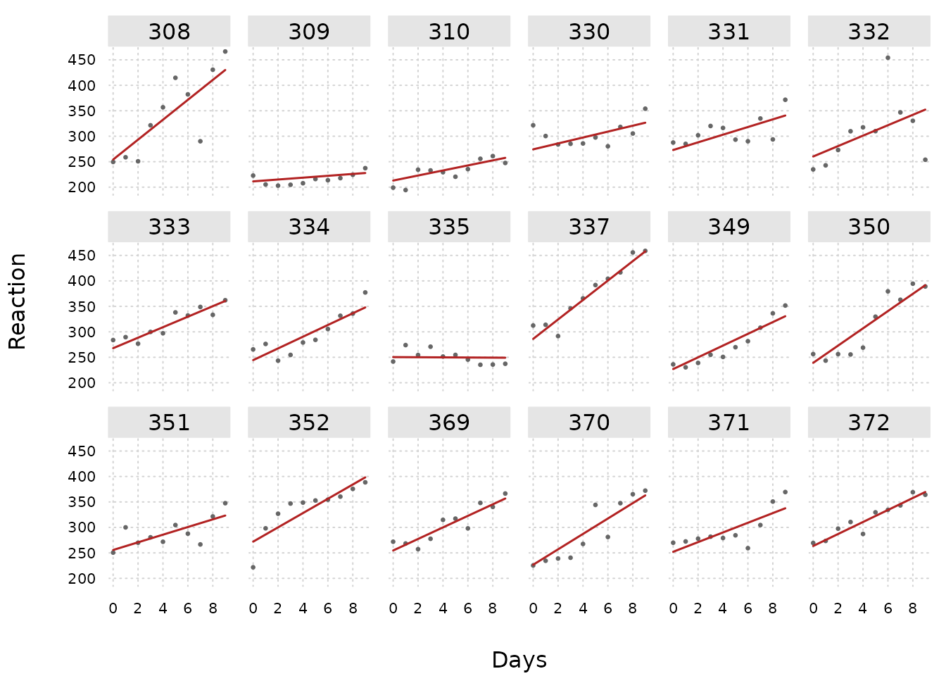
The figures on this page use tinyplot, which is a suggested package. They are skipped when it is not installed.
Distributional regression
Every distributional parameter can get its own formula with the full predictor grammar, including random effects and smooths:
fit2 <- frm(bf(Reaction ~ Days + (Days | Subject),
               sigma ~ Days), family = gaussian(),
            data = sleepstudy)
fixef_by_dpar(fit2)$sigma
#> (Intercept)        Days
#>   2.8118465   0.0846344
The coefficient on Days is positive, so the model says
that reaction times scatter more widely late in the study. Compare the
fitted residual standard deviation with the standard deviation of the
residuals on each day.
day_sd <- as.numeric(tapply(residuals(fit2)[, "Estimate"],
                            sleepstudy$Days, sd))
sig <- as.numeric(frm_linpred(fit2, dpar = "sigma", type = "response",
                          newdata = data.frame(Days = 0:9,
                                               Subject = "308")))
tinyplot::tinyplot(x = 0:9, y = day_sd, type = "p", pch = 16,
                   col = "gray30", theme = "clean2", xlab = "Days",
                   ylab = "residual standard deviation",
                   ylim = range(c(day_sd, sig)))
tinyplot::plt_add(x = 0:9, y = sig, type = "l", col = "firebrick",
                  lwd = 2)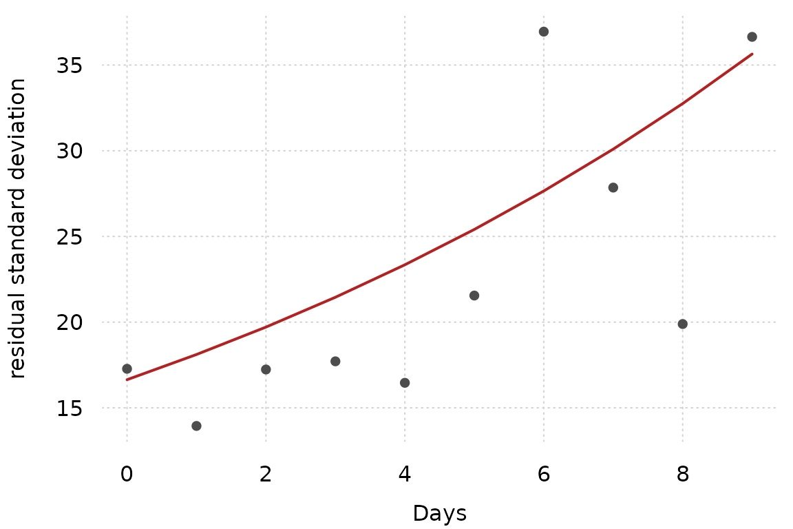
The daily standard deviations are noisy, because each one comes from 18 observations. The trend they show is the trend the model fits.
Nonlinear formulas
With nl = TRUE the model formula is an arbitrary R
expression over named parameters, each of which has its own linear
predictor:
set.seed(1)
d <- data.frame(x = runif(200, 0, 5))
d$y <- 2.5 * exp(-0.7 * d$x) + rnorm(200, 0, 0.15)
nlfit <- frm(bf(y ~ a * exp(-b * x), a ~ 1, b ~ 1, nl = TRUE) +
               gaussian(),
             data = d, start = list(beta = c(1, 0.3)))
fixef(nlfit, flatten = TRUE)
#>     a_(Intercept)     b_(Intercept) sigma_(Intercept)
#>         2.5067769         0.7022003        -1.9048113
Every nonlinear parameter starts at zero unless start or
a located prior moves it. For a monotone term that is usually good
enough. For a BUMP-SHAPED term it is not, because a bump evaluated away
from the data is flat in every one of its parameters at once. Write a
peak exp(lamp) * exp(-0.5 * ((w - pk) / exp(lsig))^2) over
w from 1 to 45 and pk starts at 0, where the
bump underflows to zero everywhere: the amplitude, the centre and the
width then have no gradient, the Hessian is singular and every standard
error is NaN. The fit is not overparameterized. It never
had a gradient to follow.
Two spellings avoid it. Put the centre where the data is, either with a start value or by writing the offset into the formula:
# start the centre in the middle of the range
frm(bf(I ~ exp(lamp) * exp(-0.5 * ((w - pk) / exp(lsig))^2),
       pk ~ 1, lamp ~ 1, lsig ~ 1, nl = TRUE),
    family = exponential("log"), data = d,
    start = list(beta = c("pk_(Intercept)" = 10)))

# or estimate a DEPARTURE from a centre you already know
bf(I ~ exp(lamp) * exp(-0.5 * ((w - (10 + pk)) / exp(lsig))^2), ...)
diagnose(fit) names the flat parameters when this
happens, under “Flat directions”.
A nonlinear parameter also cannot be named after one of the family’s
own distributional parameters. mu ~ 1 + (1 | id) in a
nl = TRUE model gives the family’s own mu a
linear predictor, and the model body then has no mu to
refer to; frm() refuses it and names the reserved set. Any
other name is free, including b and theta.
Those two are also parameter-template component names, so
start = list(b = ) still means the random-effect vector,
not the parameter: a nonlinear parameter’s coefficients live inside
beta, as
start = list(beta = c("b_(Intercept)" = 1)).
Custom families
A family is a plain R function returning an AD-safe log-density; no Stan or C++ involved:
my_poisson <- custom_family(
  "my_poisson", dpars = "mu", links = list(mu = "log"),
  lpdf = function(y, dpars, aterms) {
    y * log(dpars$mu) - dpars$mu - lgamma(y + 1)
  }
)
check_custom_family(my_poisson, y = rpois(50, 3),
                    dpars = list(mu = rep(2.5, 50)))
An inverse link saturates, so a density written over
1 - mu or log(mu) loses the tail:
plogis(eta) is exactly 1 in double precision from
eta = 36.7368 up, and there 1 - mu is exactly
0, which gives NaN for the value and for the gradient.
frm() keeps each linear predictor beside its distributional
parameter while the objective is taped, and
?"frmtmb-robust-dpars" is how a density reads it.
# a gate the optimizer has pushed against 1
d_on <- list(zi = plogis(40), .eta_zi = 40)
c(plain = log(1 - d_on$zi),
  robust = dpar_log1m(d_on, "zi", "logit"))
#>  plain robust
#>   -Inf    -40
check_custom_family() supplies no linear predictors, so
it exercises the fallback path only. Test the other one by building the
dpars list by hand, as above.
Smooths and Gaussian processes
mgcv smooths and gp() terms work in any linear
predictor; their smoothing and kernel parameters are estimated as
variance components. gp() takes up to three variables and
brms’s arguments: iso = TRUE, the default, shares one
lengthscale and iso = FALSE gives one per dimension, and
by = f fits one GP per level of a factor, with its own
standard deviation and lengthscale, or multiplies the GP by a numeric
by. The exact form predicts at new positions by kriging;
the Hilbert-space form (k =) interpolates through its
basis, capped at k^D <= 1000 columns. The Hilbert-space
form uses brms’s input convention: the coordinates are divided by their
largest pairwise distance, so the boundary factor c = (1.25
by default, one value per variable) means the same thing here as in
brms. Reported lengthscales stay in data units.
Spatial Gaussian Markov random fields
car(), brms’s conditional autoregressive field over an
adjacency matrix, and spde(), a Matern field over a
finite-element mesh, are in the extension package frmtmb.spatial. Load
it with library(frmtmb.spatial); its vignette,
vignette("spatial", package = "frmtmb.spatial"), covers
both. Without the package, frm() refuses either term by
name and says how to load it.
Special terms
mo() fits monotonic effects of ordinal predictors,
mi() imputes missing continuous predictors inside the model
(with mi(sdx) for known measurement error), and
se() gives meta-analysis:
set.seed(3)
dm <- data.frame(inc = sample(0:3, 300, TRUE), z = rnorm(300))
dm$y <- 1 + c(0, 1, 1.6, 2)[dm$inc + 1] + 0.3 * dm$z + rnorm(300)
fmo <- frm(bf(y ~ mo(inc) + z), family = gaussian(), data = dm)
frm_linpred(fmo, newdata = data.frame(inc = 0:3, z = 0))
#>         1         2         3         4
#> 0.9227854 1.8599437 2.5575758 2.9094143
Mixtures
Finite mixtures keep per-component parameters and covariate-dependent
mixing weights; groups = ~g moves the class draw to the
group level (latent classes, combinable with random effects):
mix <- mixture(gaussian(), gaussian(), groups = ~g)
dmix <- data.frame(y = 0, g = factor(rep(1:40, each = 5)))
# frm_simulate() draws one class per GROUP here, which is what
# groups = ~g means; theta1 and theta2 are the mixing probabilities,
# brms's simplex, set together
dmix$y <- frm_simulate(bf(y ~ 1) + mix, dmix,
                       newparams = list(b_mu1_Intercept = -1,
                                        b_mu2_Intercept = 2,
                                        sigma1 = 0.8, sigma2 = 0.8,
                                        theta1 = 0.6, theta2 = 0.4),
                       nsim = 1, seed = 4)[[1]]
fmix <- frm(bf(y ~ 1) + mix, data = dmix)
head(mixture_probs(fmix), 3)
#>      class1       class2
#> 1 0.9999996 3.511889e-07
#> 2 1.0000000 3.214083e-11
#> 3 1.0000000 1.006305e-14
Inference beyond Wald
hypothesis() tests arbitrary parameter expressions
(Wald, profile, or parametric bootstrap) and returns brms’s object. It
uses brms’s names: b_Days for a coefficient, which brms’s
default class = "b" lets you write Days, and
natural-scale names such as sd_Subject__Days, which need
class = NULL:
hypothesis(fit, "Days > 5")
#> Hypothesis Tests for class b:
#>       Hypothesis Estimate Est.Error CI.Lower CI.Upper Evid.Ratio Post.Prob Star
#> 1 (Days)-(5) > 0     5.47       1.5        3     7.94         NA        NA    *
#> ---
#> 'CI': 90%-CI for one-sided and 95%-CI for two-sided hypotheses.
#> Method: wald. Est.Error is the standard error; Evid.Ratio and
#> Post.Prob are NA, because a maximum-likelihood fit has no posterior.
#> '*': For one-sided hypotheses, the one-sided test rejects at level 0.05;
#> for two-sided hypotheses, the value tested against lies outside the 95%-CI.
#>      Hypothesis     z         p
#>  (Days)-(5) > 0 3.639 0.0001366
hypothesis(fit, "sd_Subject__Days^2 / (sd_Subject__Days^2 + sigma^2) = 0",
           class = NULL)
#> Hypothesis Tests for class :
#>                                              Hypothesis Estimate Est.Error
#> 1 (sd_Subject__Days^2/(sd_Subject__Days^2+sigma^2)) = 0     0.05      0.02
#>   CI.Lower CI.Upper Evid.Ratio Post.Prob Star
#> 1     0.01     0.09         NA        NA    *
#> ---
#> 'CI': 90%-CI for one-sided and 95%-CI for two-sided hypotheses.
#> Method: wald. Est.Error is the standard error; Evid.Ratio and
#> Post.Prob are NA, because a maximum-likelihood fit has no posterior.
#> '*': For one-sided hypotheses, the one-sided test rejects at level 0.05;
#> for two-sided hypotheses, the value tested against lies outside the 95%-CI.
#>                                             Hypothesis     z       p
#>  (sd_Subject__Days^2/(sd_Subject__Days^2+sigma^2)) = 0 2.389 0.01688
frm_bootstrap() runs a warm-started parametric
bootstrap, and confint(fit, method = "profile") profiles
single parameters.
Simulating from a design
frm_simulate() builds a design from a formula and data,
sets the parameters, and simulates responses - no fit needed. This is
the power analysis loop: simulate, refit, count. Parameters take brms’s
names, the strings variables() returns: b_x
for a coefficient, on the link scale; sigma as a residual
SD; and sd_<group>__<term> as a standard
deviation. A bare name such as x is refused with its brms
spelling:
set.seed(1)
dd <- data.frame(x = rnorm(120), g = factor(rep(1:12, 10)), y = 0)
form <- bf(y ~ x + (1 | g)) + gaussian()
# The draw takes its own seed, away from the chunk's: reusing
# set.seed(1) restarts the same random stream that made x, and the
# residuals come out equal to the covariate.
sims <- frm_simulate(form, dd, nsim = 3, seed = 1001,
                     newparams = list(b_Intercept = 1, b_x = 0.5,
                                      sigma = 0.6,
                                      sd_g__Intercept = 0.7))
str(sims, max.level = 0)
#> 'data.frame':    120 obs. of  3 variables:
Give prior instead and every simulation draws its own
parameter vector first - the analog of brms’s
sample_prior = "only" followed by
posterior_predict(). The drawn parameters come back as an
attribute, so a prior-predictive check can relate parameters to
outcomes:
pp <- frm_simulate(form, dd, nsim = 50, seed = 2,
                   prior = set_prior("normal(0, 1)", class = "b") +
                     set_prior("normal(0, 2)", class = "Intercept") +
                     set_prior("exponential(1)", class = "sd") +
                     set_prior("exponential(1)", class = "sigma"))
pars <- attr(pp, "pars")
head(pars, 3)
#>          b_x b_Intercept sd_g__Intercept     sigma
#> 1 -0.8969145    3.274092       0.1466527 1.7307097
#> 2  1.2004947   -1.598512       0.2034451 0.7437466
#> 3 -2.0074329    1.767528       0.4951322 0.1981281
# does the prior imply plausible data? slope against outcome spread
plot(pars$b_x, apply(pp, 2, sd), xlab = "slope", ylab = "sd(y)")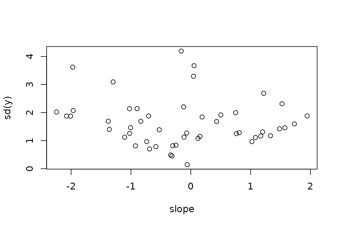
Every coefficient and every random-effect SD needs a value from
newparams or a prior; leaving one out is an error rather
than a silent zero effect.
Diagnostics
diagnose(fit) reports convergence forensics.
Simulation-based residuals come through DHARMa, predictive checks
through pp_check(), and effect displays through
conditional_effects():
plot(dharma_residuals(fit))
plot(conditional_effects(fit))
The same fitted objective can be handed to NUTS for full Bayes on the
same model. That lives in the companion package
frmtmb.sample: frmtmb.sample::frm_sample()
returns draws with the whole posterior method surface
(posterior_epred(), hypothesis(),
loo()), and frmtmb.sample::check_laplace()
audits the Laplace approximation against them.
See vignette("inputs") for what frm()
accepts and what it costs to run,
vignette("brms-migration") for the brms feature map, and
vignette("diagnostics") for the model-checking
workflow.