Diagnostics for a frmtmb fit answer three separate questions: did the optimizer find a real optimum, does the fitted family describe the data, and are the reported uncertainties trustworthy. Each has its own tool.
library(frmtmb)
#>
#> Attaching package: 'frmtmb'
#> The following object is masked from 'package:stats':
#>
#>     ar
set.seed(1)
n <- 400
dd <- data.frame(x = rnorm(n), g = factor(rep(1:20, n / 20)))
dd$y <- rpois(n, exp(0.5 + 0.4 * dd$x + rnorm(20, 0, 0.5)[dd$g]))
fit <- frm(bf(y ~ x + (1 | g)) + poisson(), data = dd)
Did the optimizer converge?
diagnose() reports the convergence code, the largest
gradient component at the optimum, whether the Hessian is positive
definite, and covariance parameters near a boundary (a variance
component collapsing to zero is the common case):
diagnose(fit)
#> Optimizer convergence code: 0 (relative convergence (4))
#> Max |gradient|: 6.943e-05 at (Intercept)
#> Hessian positive definite: TRUE
#> No convergence problems detected
Convergence problems
The warning “Large maximum absolute gradient at the optimum” means
two things at once, and the second one is the finding. The optimizer
stopped where the objective still has slope above
frmtmb_control(grad_tol = 1e-3), AND one exact Newton step
from there would still gain more than grad_tol in
log-likelihood. The warning gives that second number, so it says how
much the fit is short by rather than only that a derivative is
large.
A gradient alone cannot say this. The optimizer stops on a RELATIVE
change in an objective that grows with the sample size, so the gradient
at a perfectly good optimum grows with it too: the same gaussian design
warned on 0 of 20 replicates at 200 rows and 20 of 20 at 20,000. A
parameter sitting on a bound from set_prior(ub = ) also has
a nonzero gradient by construction, because the constrained optimum is
the bound. Neither is counted now.
The check has one blind spot, and it is worth knowing because the
remedy is a setting rather than a refit. The gradient is what admits a
fit to the second reading, so a fit whose gradient never reaches
grad_tol is never looked at. A predictor column scaled far
below one does that: it holds the gradient down while the coefficient
stalls. With autoscale = FALSE and a column spread of
1e-7 a gaussian fit reports convergence at a gradient of
1.6e-5 and a log-likelihood 297 units below the
standardized fit of the same data, silently. The default
autoscale rule is what closes it, and
diagnose() names badly scaled columns whether or not the
gradient noticed.
Work through these in order; each step tells you something even when it does not fix the warning.
-
Identify the parameter.
diagnose(fit)prints the largest gradient component and its name, the parameters a bound holds in place, the largest gradient over the rest WITH its own parameter, and the log-likelihood still on the table. On a fit with an active bound those are two different parameters, and the one beside the projected gradient is the one to work on: the other is pinned and cannot move. A coefficient of a continuous predictor points to scaling; atheta_*component points to a variance-parameter problem, anddiagnose()flags extreme values (a log-SD far below zero is a variance collapsing to its boundary, which is a model issue, not an optimizer issue). -
Fix predictor scaling. For a flagged coefficient,
frmtmb_control(autoscale = TRUE)standardizes badly scaled columns internally and judges convergence in the rescaled units; rescaling the variable in the data works equally well. -
Restart harder.
frmtmb_control(restarts = 3)re-launches the optimizer from the current optimum until the gradient passes;optCtrl = list(iter.max = 5000, eval.max = 5000)lifts the iteration caps for slow problems. -
Compare optimizers.
frm_allfit(fit)refits with nlminb, optim, bobyqa, and nloptr and tabulates log-likelihoods. All optimizers agreeing on the log-likelihood to several decimals while one warns usually means a flat ridge near the optimum, not a wrong answer; disagreement means the warning is real. -
Look at the profile.
plot(profile(fit, "theta_1"))shows whether the flagged parameter sits in a flat valley (benign) or on a slope (not converged). -
Boundary fits. When a random-effect SD is
collapsing to zero, the likelihood surface is one-sided and the gradient
check can never fully settle. Either simplify the random-effect
structure, or keep the term and regularize with
prior = set_prior("exponential(1)", class = "sd")(a MAP fit; the same move asblme’s covariance priors). -
Judge marginal cases by the log-likelihood, not the
gradient. Read the second number in the warning, which
diagnose()also prints. It is what a Newton step would gain, and it is measured on the scale answers live on: below1e-3nothing you report can move, and a warning at1e-3to1e-2is worth a look but rarely worth a refit. A large one is real, whatever the gradient reads: a near-collinear design can warn with a gradient of5e-3and half a log-likelihood unit left, which no restart recovers.frmtmb_control(grad_tol = )tunes both readings together, and steps 4-5 are the evidence for deciding.
Does the family fit the data?
Three residual types, in increasing order of statistical care:
-
residuals(fit)is response-scale (y - E[y]), in the response’s units. Good for effect-size intuition, useless as a distributional check for counts. -
residuals(fit, type = "pearson")standardizes by the family variance. -
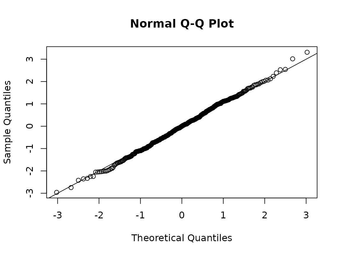
residuals(fit, type = "osa")gives one-step-ahead quantile residuals via [TMB::oneStepPredict()]: each observation’s CDF position given the previous ones, mapped through the normal quantile function. They are standard normal under a correctly specified model regardless of family, and remain valid under correlated observations, where pearson residuals mislead.
Simulation-based residuals through DHARMa cover the same ground with a richer test suite (dispersion, zero-inflation, outliers) and better plots:
dh <- dharma_residuals(fit, nsim = 200, seed = 1)
plot(dh)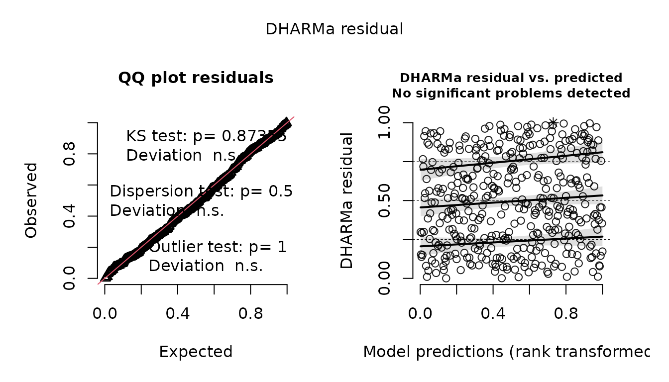
DHARMa::testDispersion(dh, plot = FALSE)
#>
#>  DHARMa nonparametric dispersion test via sd of residuals fitted vs.
#>  simulated
#>
#> data:  simulationOutput
#> dispersion = 1.0486, p-value = 0.59
#> alternative hypothesis: two.sided
A misspecified model shows up immediately; here the same data fit without the group effect is overdispersed:
fit_bad <- frm(bf(y ~ x) + poisson(), data = dd)
DHARMa::testDispersion(dharma_residuals(fit_bad, nsim = 200, seed = 1),
                       plot = FALSE)
#>
#>  DHARMa nonparametric dispersion test via sd of residuals fitted vs.
#>  simulated
#>
#> data:  simulationOutput
#> dispersion = 1.661, p-value < 2.2e-16
#> alternative hypothesis: two.sided
Two quicker looks. plot(fit) draws Pearson residuals
against fitted values and their normal QQ plot. And
pp_check(fit) overlays the observed response with responses
simulated from the fitted model, through bayesplot’s ppc_*
functions (brms users know this display):
bayesplot::pp_check(fit, ndraws = 20)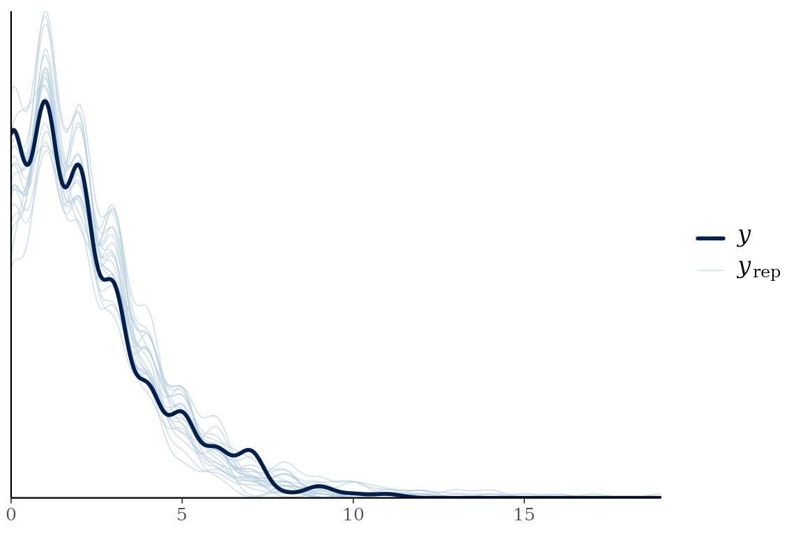
Are the standard errors trustworthy?
Wald standard errors and the Laplace approximation share failure
modes: variance components with few groups, binary data with tiny
clusters. Four things in this package route around that:
confint(method = "profile") replaces the quadratic
assumption, frm_bootstrap() replaces it with a resampling
distribution, frm(quadrature = TRUE) replaces the Laplace
approximation itself with adaptive quadrature, and
frm(importance = ) reweights it (the next section).
NaN standard errors
The covariance is the inverse of the Hessian at the optimum. Without
random effects it is the exact Hessian, from automatic differentiation.
This includes quadrature = TRUE and
importance = fits, whose outer objective has no inner
random effects. With random effects it is central differences of the
exact gradient. The step of a coefficient of a design column moves its
linear predictor by about 1e-3 in root mean square over the rows,
whatever the covariate’s units. A nonlinear parameter, a
mo() term and a variance parameter keep a step of 1e-3 on
their own scale. Where the design is ill-conditioned, the covariance
comes instead from a Hessian taken in the coordinates of the design’s QR
decomposition. A plain inverse fails as a whole: one unusable direction
makes every entry NaN. frm() does not stop
there. It builds the Hessian when it fits, and when the plain inverse
fails it tries two repairs before it gives up on a parameter:
- It scales the Hessian to unit diagonal and inverts that. This is the same matrix, so it changes nothing where the plain inverse worked. It recovers the standard errors where one parameter is on a very different scale from the others.
- When that also fails, it removes the directions the likelihood does not determine and keeps the standard errors of the other parameters. A parameter goes with a direction when a measurable part of it lies along that direction, so a direction spread over many coefficients takes all of them.
The parameters it removes have no standard error. frm()
names them in one warning, “Standard errors are not available for k of n
parameters”, with a reason for each:
- A bound holds it. The fit is a constrained optimum. The other standard errors are conditional on the bound.
- The data separate the outcomes. A coefficient of a binomial or ordinal model runs off toward infinity, and the optimizer stops where its tolerances do.
-
The likelihood is flat along it. A standard
deviation at 0 does this. So does a
mo()simplex whose steps the data read only as a sum, when a category in between has no rows. Two parameters that enter only through their sum do it too, and so does a nonlinear term evaluated outside its own support; see the nonlinear section ofvignette("frmtmb"). - A step along it raises the log-likelihood. The estimates are not a maximum in that direction. Refit from other starting values. A short step along the direction confirms this before the warning says it; a direction where the step does not gain is called flat.
- Its Hessian row is not finite.
-
The inverse gives it a variance of zero or less.
The curvature where the fit stopped does not measure the uncertainty. A
log density with a kink in a parameter does this:
asym_laplace()is piecewise linear in its location, so its exact Hessian has no curvature there.vcov()showsNaN, never 0, andsummary()gives this reason.
An earlier warning that names a parameter, such as the one for a
grouping factor with one level, explains that parameter only. The other
parameters still appear in this warning. A setting of
"ignore" on the earlier check does not explain
anything.
summary() repeats the list under the coefficient tables,
and confint() and vcov() show NaN
for those parameters only. A prediction whose standard error depends on
a removed direction gets NaN for it, and so does an emmean
or a hypothesis(). fitted(),
predict(), frm_linpred(),
conditional_effects(), emmeans() and
hypothesis() warn once per call with the number of such
rows. A prediction that does not move along a removed direction keeps
its standard error. A fit that did not converge gets the convergence
warning instead of this one, and keeps sdreport()’s own covariance.
The check costs time. On a model without random effects it reads the
exact Hessian, at about one gradient per coefficient: 8 to 23 percent of
the fit on small models and 19 to 24 percent on a model with 301
coefficients. With random effects it builds the finite-difference
Hessian, two gradients per outer parameter, when the model has at most
10 outer parameters or those gradients are at most a quarter of the
evaluations the optimizer made. Otherwise the check waits for the first
use of a standard error (summary(), fixef(),
vcov(), confint(), a prediction’s standard
error) and warns there, so a large mixed model can fit without the
warning and give it later. The rule counts work and does not read the
clock, so a call warns in the same place on every run. To skip the
check, use frmtmb_control(check_se = "ignore"). On a model
without random effects the first vcov() then builds the
exact Hessian itself. That takes less time than the finite differences
it replaces, but more memory: on a bernoulli model with 10,000 rows the
peak working set was 350 MB higher with 200 coefficients and 870 MB
higher with 500.
diagnose(fit) also reports “Flat directions” when the
likelihood does not depend on a parameter at all: zero gradient and an
empty Hessian row, measured by perturbing the parameter and seeing
whether the gradient moves.
To measure the violation rather than route around it, install the
companion package frmtmb.sample and read
vignette("posterior-diagnostics", package = "frmtmb.sample"),
which covers check_laplace() and the diagnostics of a
sampled fit; this page stays with the maximum-likelihood side.
A distributional parameter with no maximum
A standard error in the thousands on an estimate in the tens is not a wide interval. It means the likelihood was still rising where the optimizer stopped, so the number reported is the stopping point.
student()’s nu is the case you will meet. A
student-t becomes a gaussian only as nu goes to infinity,
so on data with no heavy tails the likelihood has no maximum in
nu and the fit reports whatever the last step reached.
Values above 1e9 are ordinary, and two runs of the same
model on the same data in a different row order can differ by orders of
magnitude in nu while agreeing on every coefficient.
set.seed(41)
du <- data.frame(x = rnorm(120))
# uniform errors: lighter tails than any student-t
du$y <- 1 + 0.5 * du$x + (runif(120) - 0.5) * 3.4
diagnose(frm(bf(y ~ x) + student(), data = du), quiet = TRUE)$unbounded_dpar
#>         parameter estimate std.error      value
#> 1 nu: (Intercept) 21.69349  8334.486 2638538842
diagnose() reports this as “Distributional parameter at
the end of its link” and prints the natural-scale value beside the
link-scale estimate. The pair is the evidence, not either half: a
parameter legitimately far out on its link keeps a small standard
error.
Read the fit as the gaussian one it has become. To get a number you
can report, refit with gaussian(), or hold nu
somewhere finite with a prior; see set_prior().
The same parameter runs off the other end, and there the reading is
opposite. On tails heavier than any identified nu can hold,
nu goes down to one: log(nu - 1) around -20, a
standard error in the thousands, and a natural-scale value that prints
as 1.
set.seed(77101)
dc <- data.frame(x = rnorm(200))
dc$y <- 1 + 0.5 * dc$x + rcauchy(200)      # the heaviest tails there are
diagnose(frm(bf(y ~ x) + student(), data = dc), quiet = TRUE)$unbounded_dpar
#>         parameter  estimate std.error value
#> 1 nu: (Intercept) -19.19701  4541.299     1
diagnose() names this under the same heading, so read
the sign. A large POSITIVE estimate means no heavy tails and
gaussian() says so. A large NEGATIVE one means the
opposite, and gaussian() is then the worst fit available:
the data is the message, and a prior is the way to hold nu
finite.
When the Laplace approximation is the problem
The tools above ask whether the reported uncertainty is trustworthy. This section asks whether the estimate is, because the Laplace approximation has a regime where it is biased, and no interval method repairs a biased point estimate.
The regime is the package’s named audience: a binary response in small clusters. The Laplace approximation replaces each group’s integral by a Gaussian centered on the conditional mode. For a Bernoulli response with a handful of rows per group, the integrand is skewed, the Gaussian does not match it, and the variance component comes out too small.
frm(importance =) corrects that. It keeps the Laplace
Gaussian, but uses it as a proposal: it draws from it,
reweights the draws by how much the true integrand differs from it, and
averages. The result is an unbiased estimate of the exact marginal
likelihood, at every parameter value, not an approximation that is
accurate only near the optimum. The method is Skaug and Fournier’s
(2006), and it is what ADMB’s -is option does.
set.seed(7)
ng <- 40
per <- 5
gg <- rep(seq_len(ng), each = per)
xx <- rnorm(ng * per)
bb <- cbind(rnorm(ng, 0, 1.5), rnorm(ng, 0, 1))
bd <- data.frame(
  y = rbinom(ng * per, 1,
             plogis(-0.5 + 0.8 * xx + bb[gg, 1] + bb[gg, 2] * xx)),
  x = xx, g = factor(gg)
)
Fit it both ways. The correction takes a draw count, and 0 (the default) turns it off:
lap <- frm(bf(y ~ x + (x | g)) + bernoulli(), data = bd)
imp <- frm(bf(y ~ x + (x | g)) + bernoulli(), data = bd,
           importance = 500)
c(laplace = as.numeric(logLik(lap)),
  importance = as.numeric(logLik(imp)))
#>    laplace importance
#>  -119.5584  -118.4071
The corrected log-likelihood is the honest one. print()
says so, and says how far it can be trusted:
imp
#>  Family: bernoulli
#>  Links: mu = logit
#>
#> Formula: y ~ x + (x | g)
#>    Data: bd (Number of observations: 200)
#>  Method: ML   logLik: -118.407   AIC: 246.814   BIC: 263.306
#> Marginal likelihood: importance-corrected, 500 draws per group in 2 rounds (MCSE 0.12, min ESS 0.63 of 1)
#>
#> Multilevel Hyperparameters:
#> ~g (Number of levels: 40)
#>                  Estimate Est.Error l-95% CI u-95% CI
#> sd(Intercept)        1.10      0.41     0.53     2.27
#> sd(x)                2.46      0.74     1.37     4.43
#> cor(Intercept,x)    -0.06      0.40    -0.69     0.62
#>
#> Regression Coefficients:
#>           Estimate Est.Error l-95% CI u-95% CI z value Pr(>|z|)
#> Intercept    -0.77      0.30    -1.36    -0.18   -2.57     0.01
#> x             1.17      0.54     0.11     2.23    2.17     0.03
Note what this model is. The random effect is a correlated intercept
and slope, so the per-group integral is two-dimensional.
quadrature = TRUE cannot marginalize it at all: the
Gauss-Kronrod transform underneath it integrates one scalar random
effect at a time. The importance correction takes any block dimension,
which is the main reason to reach for it.
Reading the effective sample size
An importance estimate is only as good as the proposal’s coverage of the integrand. The effective sample size measures that coverage, one number per group, as a fraction of the draws:
summary(imp$importance$ess)
#>    Min. 1st Qu.  Median    Mean 3rd Qu.    Max.
#>  0.6252  0.8247  0.8888  0.8681  0.9330  0.9913
imp$importance$mcse
#> [1] 0.1150382
Read it like this.
- Near 1 means the weights are nearly equal, so the proposal matches the integrand and almost every draw is doing work. For a gaussian response it is exactly 1, because the Laplace approximation is already exact and there is nothing to reweight.
- Below
0.25the fit warns and names the groups. That threshold is placed by measurement, not by taste. Ordinary designs sit far above it: 0.93 on the package’s probe design, 0.97 on a scalar random intercept, exactly 1.00 for a gaussian response, 0.63 here. Forty groups of three binary rows with a standard deviation of two report 0.28 to 0.90, depending on the sample. A proposal that has stopped working sits below it. On thirty groups of two binary rows with a correlated slope, the worst group at 500 draws runs from 0.02 to 1 over ten data sets: the tail of a group’s integrand can be wider than the Gaussian’s. -
mcseis the Monte Carlo standard error of the corrected log-likelihood, derived from those effective sample sizes. It is a rough scale, because it can read high or low. It counts each draw as independent, and the draws come in antithetic pairs. Over 40 seeds at 200 draws, a binomial model reads 0.0044 where the error’s standard deviation is 0.0017, so the number is too high. On a heavy-tailed or nearly even weight it is too low by a factor of 1.2 to 2: a Student response withnu = 5, 15 groups of 6 and 1000 draws has an error whose standard deviation is 1.3 to 1.4 times the number, a nominal 95 percent interval covers 0.86, and none of 100 fits warned.
To judge whether two corrected fits really differ, do not rely on
mcse alone. Refit with another
frmtmb_control(importance_seed =), or with twice the draws,
and read how far the log-likelihood moves.
If the warning fires, raise importance. The estimate
stays unbiased either way; what degrades is precision, and the effective
sample size is what tells you so.
What it costs
The correction tapes N stacked copies of the likelihood,
so time and memory grow linearly in the draw count. On a 480-row,
two-dimensional block with 60 groups, the gradient costs about 0.35 ms
per draw against 3.3 ms for the Laplace gradient. A thousand draws on
that model is a few seconds. Start at a few hundred draws, read the
effective sample sizes, and raise the count only if they ask for it.
Center a column whose mean is more than about 1e4 times its standard deviation. At 2e4 times, six of eight ordinal fits warned of false convergence, with their standard errors not available, and one moved a slope by 0.13 standard errors with no warning.
The fit proceeds in rounds. Each one anchors a proposal at the
current estimate, optimizes, and anchors again at the result; the loop
stops when the estimates settle, usually after one or two rounds. The
standard normal draws stay fixed. While the optimizer moves, the
proposal’s mode and variance move with the parameters, to first order
around the anchor, so the objective is smooth and its curvature is close
to that of the exact integral. frmtmb_control() holds the
seed, the round cap and the effective-sample-size threshold. The seed
makes the fit reproducible to the last bit, and the draws come from a
private random stream, so a fit neither reads nor disturbs the session’s
random state.
If a draw count is too small for a model, the fit stops. The message gives the worst group’s effective sample size and a larger count at which the same fit settled, or says that no larger count settled.
Scope
The correction takes any number of random-effect blocks, of any
dimension, if they share one grouping factor with one set of levels.
That is what distributional regression writes: (1 | g) in
mu and (1 | g) in sigma are two
blocks over g, and a level’s coefficients from both are
drawn together from one proposal. Blocks over different
factors, crossed or nested, are refused by name, because the marginal
likelihood is then one integral over every factor at once and does not
split into the per-group integrals the correction resamples. The
response must be a single one whose family has a rowwise density.
trunc() and cens() are supported, which is a
real difference from quadrature = TRUE: that method has to
refuse truncation because its far quadrature nodes underflow the
truncation normalizer, while importance draws stay near the conditional
mode. Truncation does not degrade the correction either. Walking a bound
up past the response median, discarding 64 percent of the rows, still
leaves the worst group holding 0.60 of its draws. Everything outside the
scope is refused by name, with the remedy in the message.
frm_compat("importance") lists the rules.
Variance components on their natural scale
confint_varcorr() reports random-effect SDs and
correlations with delta-method intervals on interpretable scales:
confint_varcorr(fit)
#>   block        term type  estimate       lwr       upr
#> 1 1 | g (Intercept)   sd 0.4783034 0.3383263 0.6761937