Conditional effects of predictors — conditional

For each requested effect, predicts over a grid of that predictor with every other predictor held at a reference value (numeric: mean; factor: first level; matrix covariate: column means) and random effects excluded (re_formula = NA). Confidence bands are Wald intervals computed on the link scale and back-transformed. Smooth terms are part of the predicted curve; conditional_smooths() draws each smooth term on its own, as brms's function of that name does.

Usage

conditional_effects(x, ...)

# S3 method for class 'frmtmb_fit'
conditional_effects(
  x,
  effects = NULL,
  resp = NULL,
  dpar = NULL,
  resolution = 100,
  prob = 0.95,
  method = c("epred", "predict"),
  band = c("wald", "profile", "boot"),
  re_formula = NA,
  ndraws = 400,
  boot = NULL,
  profile_points = 25,
  seed = NULL,
  conditions = list(),
  surface = FALSE,
  spaghetti = FALSE,
  select_points = 0,
  too_far = 0,
  data = NULL,
  int_conditions = list(),
  categorical = NULL,
  ...
)

Arguments

x: A frmtmb_fit.
...: allow_new_levels, passed to predict.frmtmb_fit(). Anything else is reported as unknown, by name, against conditional_effects().
effects: Character vector of variable names, or "x:z" pairs; for a pair, the first variable is varied over its range while the second is held at its levels (factors) or at mean and mean plus or minus one SD (numeric). Default: every fixed-effect and smooth variable of the selected linear predictor, plus one "a:b" pair per fitted interaction (brms's default); a term of order three or more contributes its leading pair. A named effect is valid when each of its variables is one the model reads (a predictor of any parameter, or a grouping variable), as in brms. An invalid effect among valid ones is dropped with brms's warning "Some specified effects are invalid for this model", and when none is valid the call stops with brms's "All specified effects are invalid for this model". A variable that is in the data but not in the model is invalid.
resp, dpar: Response and distributional parameter, as in predict.frmtmb_fit().
resolution: Number of grid points for a varied numeric predictor.
prob: Coverage of the confidence bands (brms spelling).
method: "epred" (default): Wald bands for the expected response, which for a family whose mean is not the inverse link of its mu predictor (zero-inflated, hurdle, trials(), truncated) is the MEAN and not that predictor. brms's own spellings "posterior_epred" and "posterior_predict" are accepted as aliases. "predict": prediction intervals - quantile bands from ndraws responses simulated from the family at each grid point (observation noise; random effects stay excluded, as in brms with re_formula = NA), with estimate__ the MEDIAN of the same draws, as brms reports the median of its predictive draws: on the scale of the draws (a count under trials(), inside the bounds under trunc()), and a whole count for a discrete family when ndraws is odd. It is not the expected response, which method = "epred" shows. The draws respect the response's addition terms. As in brms, a trials() variable that conditions does not set is held at 1, and the variable of an se() term or a trunc() bound at its mean, like every other variable. An expression bound is evaluated on the grid, where the response is at its mean too, so trunc(lb = min(y) - 1) is mean(y) - 1. Set the variable in conditions for a bound of your choice. On the draws of frmtmb.sample::frm_sample(), "predict" draws one response per grid row and posterior draw, at the parameters of that draw, so the band is the posterior predictive band that brms draws: under the draws method's default robust = TRUE, estimate__ is its median and se__ its MAD. There, as in brms, transform applies to the predicted draws before they are summarized, with brms's warning that the argument is deprecated, and seed fixes the simulation.
band: How the confidence band is built: "wald" (default, the delta method on the scale the band is symmetric on), "profile" (likelihood-root inversion per grid point) or "boot" (parametric-bootstrap percentiles). See the band section. Only for method = "epred".
re_formula: The population switch, in brms's spelling: NA (the default) draws the population-level curve, NULL conditions on a NEW, unobserved group, and a one-sided formula keeps the named terms for one. NA removes the (x | g) group-level terms and keeps every SMOOTH, as brms does, so on a model with s(x, g, bs = "fs") the drawn curve is the grouping factor's reference level's, that being where the display holds a predictor it is not varying. A new group's conditional modes are zero, so its curve IS the population curve and what the group costs is spread: the band carries the random-effect variance on top of the coefficient uncertainty, and the grouping column of the returned frame is NA to say which group it is. band = "boot" carries it too, by drawing that group's effects once per bootstrap replicate rather than by adding a variance. To condition on an OBSERVED group, name it in conditions (conditions = list(g = "3")) or vary it as an effect (effects = "x:g"). The rule is brms's, whose display predicts with allow_new_levels = TRUE: per grid row and per group-level term, the term reads its fitted effects where every one of its grouping variables is set to a level the fit saw, and a NEW level everywhere else, which covers a variable left unset or NA, a level the fit never saw ("99", which the frame keeps), and a nested (1 | g / h) with g set and h unset, where g's effect is read and a new g:h level is drawn within it. Each distinct new level is drawn once per replicate (per posterior draw on draws) and shared by the rows and panels that name it. brms draws a new group's random effects afresh from the fitted covariance in every posterior draw, so its curve is stochastic around this one; a maximum-likelihood fit has the mode and the variance instead of draws. predict.frmtmb_fit() spells the same setting the same way; lme4's re.form is refused and says so. band = "profile" exists only for the population-level curve.
ndraws: Simulated responses per grid point for method = "predict". For the draws method: how many evenly spaced posterior draws the curves are computed over (default all).
boot: For band = "boot": NULL (default) runs one frm_bootstrap() of 200 refits and says so, a number runs that many, and a frmtmb_boot object from an earlier identical call (attr(ce, "boot")) is reused without refitting anything.
profile_points: For band = "profile": how many points of a numeric grid are profiled, the band being interpolated between them on the link scale.
seed: Seed for band = "boot", passed to frm_bootstrap().
conditions: Named list overriding reference values, e.g. list(x2 = 1, g = "b"); or a data frame whose rows define multiple condition sets (brms style), labeled by a cond__ column from its row names.
surface: TRUE draws a two-variable effect "x1:x2" of two numeric predictors as a surface: both vary over their range at resolution values each, effect2__ stays numeric, and plot() draws an image with contours. brms's argument, with brms's meaning. FALSE (the default) varies the first predictor at three values of the second.
spaghetti: TRUE adds one curve per draw as the attribute "spaghetti" of an effect whose first predictor is numeric: the grid once per draw, stacked, with that draw's curve in estimate__ and its id in sample__, as brms lays it out. A maximum-likelihood fit has draws only under band = "boot", where a draw is one refit; with any other band it is refused. It cannot be combined with surface = TRUE.
select_points: For plot(points = TRUE): 0 (the default) draws the observations the faceting section describes. A positive number also drops each observation whose value of a numeric predictor is farther than this from the value the curve holds that predictor at, both scaled to the unit interval over the observed range. brms's argument; the points are in the attribute "points".
too_far: For surface = TRUE: remove the grid points farther than this from every observation, on the unit square, with mgcv::exclude.too.far(). 0 (the default) keeps all.
data: The original model data. Only needed when the model frame does not store a raw variable (e.g. a variable used only inside poly()).
int_conditions: Named list giving the values one or both variables of an effect are evaluated at, in place of the defaults (the range of a numeric grid, mean +/- sd for a numeric moderator). An element is either the values themselves or a function of the observed column, e.g. int_conditions = list(z = c(-1, 0, 1)) or list(z = function(v) quantile(v, c(0.1, 0.9))). Names on a numeric vector become the moderator's effect2__ labels. brms's argument, with brms's meaning.
categorical: Per-category display for a polytomous family: TRUE (the default there) draws one curve per response category and keys the effect "x:cats__", as brms's categorical = TRUE does; FALSE draws the expected CATEGORY NUMBER, sum(k * p_k), which is brms's default. Only for an ordinal or categorical family with no dpar; a nominal family has no ordered categories to average and refuses FALSE.

Value

A named list of data frames (one per effect), in brms's column layout: the varied variable(s), then every other model variable at the value it is held at, then cond__ (the condition label, always present), effect1__ and, for a two-variable effect, effect2__ (the moderator as a display label: rounded to two decimals, levels descending), then estimate__, se__ (on the displayed scale, as in brms), lower__ and upper__. Printing it draws the plots. A polytomous fit adds a cats__ column, one block of rows per response category, and keys the effect "x:cats__". plot(ce, points = TRUE) overlays the raw observations (the brms argument), each panel showing only the observations that belong to its own condition; see the faceting section. No points are drawn for a per-category ordinal display, a non-mean dpar, or a matrix response (a message says so).

New rows of a model with me()

A grid row has no latent value. The estimate is the value at the held x, which is close to the median of brms's draws, and se__, lower__ and upper__ carry the variance of the draw from N(x, sdx), so they are not coefficient uncertainty alone. The band is the draw's own quantiles on the response scale. A me(gr = ) group is held at NA, as brms holds it, so each grid row is a level of its own.

With several responses, the panels are in brms's order: the effects outside, over what any response reads, and the responses inside.

Several conditions become one faceted page

A conditions data frame of several rows gives the effect one panel per row, laid out as small multiples on a SINGLE page with a shared scale, the way brms's facet_wrap("cond__") does. plot(ce, ncol = ) sets the number of columns; the default lays the panels out roughly square, as brms's ncol = NULL does.

The panels are drawn with tinyplot when it is installed, which supplies the shared axes and a single outer legend. Without it the fallback is a grid of ordinary base-graphics panels, still one page and still honoring ncol, labeled by condition on the y axis. The per-category ordinal display always takes the fallback grid: its grouping slot already carries the response category.

points = TRUE draws only the observations belonging to each condition, matching brms's make_point_frame(). A condition claims the rows of the data that MATCH it on the variables it sets, so with one condition per level of a factor each observation appears once, in its own panel. Two rules bound that, both as in brms:

A NUMERIC condition variable is dropped from the match, because a reference value such as list(x2 = 0.37) is a point on a continuum that names no observation; matching on it would empty every panel. A grouping factor stored as a number is exempt, being a label rather than a continuum. A condition left with nothing to match on therefore claims EVERY observation, and its panel differs from the others only in its curve.
A condition variable that names no column of the model data cannot select anything either, so the points are left unsplit and every panel draws all of them.

Unlike brms, a variable the conditions data frame does not set is not silently pinned to its first level for this purpose, so an unmentioned factor does not drop observations from every panel.

Ordinal responses

cumulative(), sratio(), cratio() and acat() have no mean, so the display is per CATEGORY, as brms's categorical = TRUE is: each effect data frame gains a cats__ factor of the response's own levels and carries the fitted category probability in estimate__, with one curve per category in the plot (a second predictor gets a panel of its own). A one-variable effect is keyed "x:cats__" there, brms's key for that layout.

That is the DEFAULT here and it is brms's non-default: brms's own default summarizes the categories into an expected category number and warns that it is treating an ordered factor as continuous. categorical = FALSE asks for that summary anyway, sum(k * p_k) with its own delta-method band (the category weights go on the gradient, so the covariances between the category probabilities are kept), keyed "x" and directly comparable with brms's default curve. It gives brms's warning, "Predictions are treated as continuous variables", because the display is the one brms warns about; the default display gives none, because it treats nothing as continuous.

se__ is then on the probability scale, and the band is a Wald interval on the logit of the probability so it cannot leave [0, 1]. The standard errors are the delta method over the joint covariance of the coefficients, the thresholds AND the cs() coefficients: a category probability depends on all of them, and holding the thresholds fixed would understate every band.

method = "predict" is refused there (the category probabilities are already the whole predictive distribution). Naming a distributional parameter, dpar = "mu", opts back into the ordinary display of the latent linear predictor.

Confidence bands

band picks how lower__ and upper__ are found. The estimate is the same curve in all three cases; only the band changes.

"wald" (default, and free): the delta-method standard error, back-transformed from the scale the band is symmetric on. For the ordinary display that scale is the link scale. For the expected response of a family whose mean runs through several distributional parameters (zero inflation, a hurdle, trials(), truncation) the standard error is the delta method over EVERY predictor's coefficients jointly, so the cross-parameter covariances are in the band; the band's scale is then the mu link's if the mean lives on it, the log scale if the mean is positive (so the band cannot cross zero), and the response scale otherwise. The two rules agree exactly wherever the mean IS the inverse link of mu.
"profile": one likelihood-root search (TMB::tmbroot()) per grid point. A grid point's linear predictor is a linear combination of the coefficients, so the search inverts the likelihood ratio along that combination; the link is monotone, so the two endpoints map through it. The band is not symmetric and does not assume a quadratic log-likelihood, which is what makes it worth its cost near a boundary or at a small sample size.
"boot": percentiles of the grid predictions across ONE parametric bootstrap of refits, run as frm_bootstrap() runs it. One bootstrap serves every effect, condition set and ordinal category of the call; attr(ce, "boot") returns it, and passing it back as boot = costs no refits at all. The responses are simulated with every smooth, gp() and hsgp() curve held at its fit, a smooth indexed by a grouping factor included, as frm_bootstrap() holds them: brms's band is the posterior of the smooth coefficients, not their prior. A group-level term is redrawn fresh, unless the grid reads it at an OBSERVED level (see re_formula): then it is held at its fitted effects too, so that every refit estimates the same group again; responses simulated with fresh effects for it would make the refit's level a different group each time and center the band on the population curve. A term the grid reads at an observed level in some rows and at a new level in others needs both simulations at once, and that call is refused by name; band = "wald" answers it. Draws taken under re_formula = NULL carry a new group's effects and draws taken without it do not, and draws simulated with a group held are not draws simulated with it redrawn, so boot = refuses either swap by name rather than returning the wrong band.

A Student-t random-effect block enters either band as a GAUSSIAN with the t variance, nu / (nu - 2) times the scale matrix: the delta method has no other shape to offer, and the bootstrap draws the same way so that the two bands stay comparable. It is the right variance around a heavier-tailed truth, not the right quantile.

se__ is on the displayed scale, as brms's MAD of its draws is. For "wald" and "profile" it is the delta-method standard error of the displayed value: the profile changes the endpoints, not the standard error. For "boot" it is the standard deviation of the bootstrap draws. The Wald band is symmetric on the link scale, so se__ is not its half width.

The three bands answer the same question and need not give the same interval. Wald and bootstrap agree in the middle of a grid, and the remaining difference there is the bootstrap's own Monte Carlo error: on a zero-inflated fit the widths differ by 13% at 200 refits and 4% at 800. At the ENDS of a grid where the estimate is poorly determined they need not converge at all: on a steep zero-inflated shape the Wald band stays about 28% wider at 3000 refits, because it is symmetric on its own scale and the percentile band is not. The point estimate is the same curve either way.

Cost, and how it is capped. A root search is two constrained optimizations, so band = "profile" profiles at most profile_points (default 25) of a numeric grid, spread over its range and including both ends, and interpolates the endpoints linearly between them on the link scale. resolution still governs the estimate curve. A factor grid is profiled at every level. Points whose search does not converge become NA and one warning names how many. band = "boot" costs its refits once, however many effects are asked for.

Refusals. band other than "wald" needs method = "epred": a prediction interval is already a simulation quantile. band = "profile" additionally needs the displayed quantity to BE a linear combination of the parameters, so it is refused (naming "boot") for an ordinal category probability, for an expected response that runs through several distributional parameters or through truncation bounds (dpar = names one predictor and opts back in), for a nonlinear predictor, for a predictor carrying s(), gp() or hsgp() (basis coefficients are inner parameters), and for a REML fit or frmtmb_control(profile = TRUE) (the coefficients are not outer parameters there).

A nonlinear predictor (nl = TRUE) gets its "wald" band from the Jacobian of the nonlinear body, which frm_lp_basis() tapes: the delta method on the link scale, back-transformed, as for a linear predictor. On y ~ a * exp(b * z) fitted to 150 rows the standard error agreed with the standard deviation of 20000 curves drawn from the fit's covariance to within that Monte Carlo error. It is a first-order approximation, which is a stronger assumption for a curved body than for a linear one; band = "boot" makes none. The Wald band is refused for a nonlinear display that runs through several predictors (the expected response of a zero-inflated or hurdle family, a reported mixing weight, the ordinal categories) and at a new level of a term the displayed predictor itself reads, where the Jacobian of one predictor is not enough; band = "boot" covers both. band = "profile" stays refused. The per-category display of a nominal family has no Wald band either, since its probabilities have no threshold Jacobian to differentiate.

New group levels

Under re_formula = NULL, or a formula that keeps a term, each grid row reads each group-level term at an observed level or at a new level (see re_formula). Some terms read a row in their own way:

gr(g, by = f) is one term per level of f. A row reads only the term of its own f level. With g unset, the row reads a new level of that term, drawn with the covariance of that f level, as brms draws it.
mm(g1, g2) has one grouping variable per member. An unset member is NA and reads a new level. Members with the same new value (for example, two unset members) read one new level, and their weights add, as in brms. Members with different unseen values ("99" and "98") read different new levels, each drawn on its own, as two unseen levels of (1 | g) are. brms 2.23.0 gives them one shared draw, because it numbers unseen values per member, not by value. With band = "boot", a row with one member at an observed level and one at a new level of the same block is refused by name, as are rows that mix the two.
mm(g1, g2, by = cbind(f1, f2)) is one block per by-level. A member at an observed group reads the block that holds the group, and a new member reads the block of its own by-value, where its new level is drawn with that by-level's covariance. Two new members with the same value and the same by-value read one new level, and their weights add. brms 2.23.0 cannot draw a new level of such a term; it stops.
A factor-smooth (s(x, g, bs = "fs")) or a smooth with a by factor has no curve for a level that the fit did not see. When conditions sets such a factor to an unseen level, or the grid leaves it unset, the call is refused by name. brms also refuses the unseen level.

With band = "boot" and on draws, a new level is drawn as follows. The rows are predicted at a placeholder level of the term, and the draw replaces the effects of that level. The placeholder can change only a grouping column that no other part of the model reads: not a column of a fixed effect, a smooth, a by variable or a nonlinear body, and not a column of a term that the same rows read at an observed level. Two terms that both read a new level in the same rows can share a placeholder column (for example mm(g1, g2) beside (1 | g1)), because their effects are separate coefficients. If no placeholder moves the rows without moving such a column, the rows keep their columns and the term's level is renamed instead: in a copy of the fit used for those rows alone, one level of the term takes the label the rows carry, and the draw replaces its effects. That is how crossed terms such as (1 | g) + (1 | h) + (1 | g:h) are drawn when g and h are set to observed levels that the data never has together: g and h keep their levels, and g:h reads a new level. With one new level in the call, the band on draws equals brms's at the same draws and the same seed, with sample_new_levels = "gaussian" (dev/ceplot-crossed-brms.R); with several, brms draws level by level and this draw by draw, so the bands agree in law but not number. A row whose grouping variable is unset there has no label to rename to, and is refused by name. A multi-membership member that no placeholder serves is still refused by name ("cannot draw a new level of the group-level term"); then set the members in conditions to levels the fit saw, or use re_formula = NA.

Draws objects

On a frmtmb_draws object from frmtmb.sample::frm_sample() the same grids are evaluated once per posterior draw, and estimate__, lower__, upper__ and se__ are the pointwise median, quantiles and median absolute deviation of the drawn curves under brms's default robust = TRUE (the mean and standard deviation under robust = FALSE). spaghetti = TRUE keeps the curves themselves. There is no band = or method = to choose (the band IS the posterior quantile band), a nonlinear predictor and a nominal per-category display work without a delta method, and the method runs on formula-route draws that have no maximum-likelihood fit behind them. ndraws thins the draws evenly for a cheaper curve. Draws from a sampling run with laplace = TRUE are refused: the sampled vector no longer aligns with the model's parameter template.

Which predictors are plotted by default

Every variable of the selected linear predictor that the display can vary: its fixed-effect terms, its smooth terms and its mo() terms (whose design columns are placeholders, so the variable is read from the term itself). On a nonlinear fit they live one level down - the covariates the nonlinear formula reads, plus the terms of each nonlinear parameter's own predictor - and all of those are collected too. Matrix-valued columns are excluded, a grid over a matrix covariate not being a curve. Every fitted interaction whose components are single plottable variables adds an "a:b" display, as in brms: a fitted interaction hidden by default invites reading the main-effect curves as the whole story. The display takes two variables, so a three-way or deeper term contributes its leading pair, with the remaining variables at their reference values until conditions = pins them. Naming effects = overrides the search.

A response whose predictor reads mi(x, idx = ) is refused by name. Such a term reads x on the row whose index() value equals the row's idx value, and a display grid holds both at one reference value, so every grid row names the same row. brms 2.23.0 stops on the same grid. Predict over rows you build, with fitted(newdata = ).

Examples

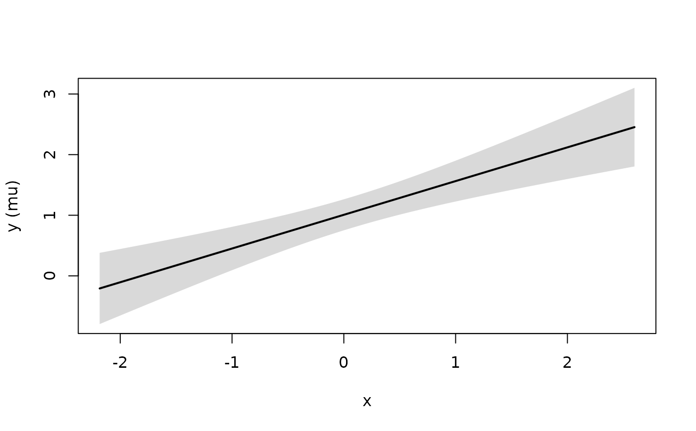
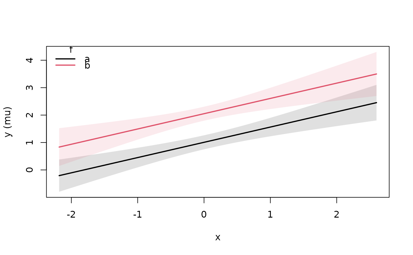
set.seed(5)
dd <- data.frame(x = rnorm(120), f = factor(rep(c("a", "b"), 60)))
dd$y <- rnorm(120, 1 + 0.5 * dd$x + (dd$f == "b"), 1)
fit <- frm(bf(y ~ x * f), family = gaussian(), data = dd)
ce <- conditional_effects(fit, effects = c("x", "x:f"))
plot(ce, ask = FALSE)


# prediction intervals instead of epred bands
ce_p <- conditional_effects(fit, effects = "x", method = "predict")
# \donttest{
# a likelihood-profile band: asymmetric, and no quadratic assumption
ce_pr <- conditional_effects(fit, effects = "x", band = "profile",
                             resolution = 20, profile_points = 5)

# a bootstrap band, reused for a second effect without refitting
ce_b <- conditional_effects(fit, effects = "x", band = "boot",
                            boot = 25, seed = 1)
ce_b2 <- conditional_effects(fit, effects = "x", band = "boot",
                             boot = attr(ce_b, "boot"))
# }