Residuals from a frmtmb fit

"osa" gives one-step-ahead (conditional quantile) residuals via TMB::oneStepPredict(): standard-normal under a correctly specified model, valid under correlated observations where pearson residuals mislead. With no group-level term, a residual of the default route is the randomized quantile residual of the fitted distribution: qnorm(F(y)) for a continuous response, and for a count qnorm(u) with u drawn uniformly on [F(y - 1), F(y)]. The uniforms are TMB's: set.seed(123) by default, so the same fit gives the same residuals and the session's random stream is left as it was; pass seed = (through ...) for other draws, or seed = NULL for the session's stream. A residual is read in the tail its row lies in, so it holds far out on either side (about +-37 and beyond).

Usage

# S3 method for class 'frmtmb_fit'
residuals(
  object,
  type = c("response", "ordinary", "pearson", "deviance", "osa"),
  osa_method = NULL,
  ...,
  ndraws = NULL,
  draw_ids = NULL,
  sort = FALSE,
  summary = TRUE,
  robust = FALSE,
  probs = c(0.025, 0.975),
  newdata = NULL,
  resp = NULL,
  allow_new_levels = FALSE
)

Arguments

object: A frmtmb_fit.
type: "response" (brms spells the same thing "ordinary", and both are accepted), "pearson", "deviance", or "osa". brms's residuals() takes newdata in this position; this one has always taken type there, so give newdata by name.
osa_method: Method for TMB::oneStepPredict(). The default is "cdf" for an uncensored core family with a CDF: each row is read against its family's own CDF, inside its own trunc() window, and a count is randomized over its own step of that CDF. An untruncated, unweighted gaussian() defaults to "fullGaussian", which is exact for a gaussian response. A censored, ordinal or CDF-less response uses "oneStepGeneric", with the integration domain and discrete support taken from the trunc() bounds or the censoring window, which must then be the same for every row. On a count, "oneStepGeneric" needs a finite discreteSupport, and the gaussian methods are refused. "fullGaussian", if asked for on a weighted fit, reads a weight as a precision, (y - mu) sqrt(w) / sigma, rather than as a frequency. A fit with quadrature = TRUE is refused: its objective has integrated the random effects already.
...: For type = "osa": passed to TMB::oneStepPredict(), and checked against that function's own formals. For every other type: refused, naming the argument. The residuals.brmsfit() arguments this one does not have (re_formula, method) are refused with the reason rather than reported as unknown names.
ndraws: brms's number of posterior draws to summarize. A maximum-likelihood fit has no Monte Carlo error to reduce, so it is accepted, changes nothing, and a message says so, as in fitted.frmtmb_fit().
draw_ids, sort, summary, robust: brms's arguments. Each needs posterior draws and a maximum-likelihood fit has none, so each is refused by name with the reason. The default of each is accepted and changes nothing.
probs: Probabilities of the two quantile columns, the ends of the Wald interval at those probabilities.
newdata: Optional data frame holding the response and the predictors: the residual is its response minus fitted(newdata = ), with that fitted value's standard error, as brms's is. Only the "response" type is defined there.
resp: For a multivariate fit: the responses to report. NULL (the default) reports all of them, as brms's n x 4 x nresp array with the third dimension named by response.
allow_new_levels: With newdata: a grouping level the fit never saw is predicted as fitted.frmtmb_fit() predicts it, instead of an error.

Value

brms's summary matrix: n rows with NULL dimnames, as brms's are, and the columns Estimate, Est.Error and one per entry of probs, NA on censored rows. The observed response is fixed, so Est.Error is the standard error of the fitted value; a "deviance" or "osa" residual has none and reports NA there. A multivariate fit asked for more than one response gives an n x 4 x nresp array, as brms's does; "osa" is univariate only.

Details

With a group-level term, TMB integrates the random effects of each one-step predictive by the Laplace approximation, and that is approximate. Against the exact one-step predictive, by quadrature on 20 groups of 10 rows (three data sets per family), the median error was below 0.001 under (1 | g) on seven count families and 0.006 to 0.016 under a latent ar() on poisson and the zero-inflated and hurdle counts. The largest was 0.15 under (1 | g) and 0.13 under ar(). The error is largest on the first row of each group, whose predictive is an integral over the group effect's prior alone. Over many rows the residuals stay calibrated: their Kolmogorov-Smirnov p-value against N(0, 1) was within 0.13 of that of the exact residuals on each of 42 fits. Read a single residual near a cutoff with that error in mind.

A case weight is a frequency, as weights() is in the likelihood (brms's reading): a row of weight w gets the residual of the last of w copies of it, given the other w - 1, and the later rows are conditioned on all w copies. A row of weight 0 is no part of the fitted likelihood and gets NA. A weight between 0 and 1 also gets NA, with a warning: there TMB reads the row's mass from the weighted density, p^w, so a count's randomization would be wrong. A residual that oneStepPredict() cannot form is NaN with a warning.

The cost grows faster than the number of rows: TMB makes three evaluations of the whole objective per row, each with an inner optimization when there are random effects. The rows are handed to oneStepPredict() in blocks of about sqrt(n), each conditioned on the rows before it, so that the objective carries the CDF of one block at a time. With (1 | g) and 2000 rows in 100 groups, poisson residuals took about a minute and negbinomial ones about two, on a loaded machine.

On a trunc()ed response, "response" residuals are taken against the truncated mean E[Y | lb <= Y <= ub]. "pearson" divides by the untruncated family variance, so it is conservative there. "osa" builds its conditional CDF on [lb, ub] (see osa_method).

On a cens()ed response, "osa" returns NA for every censored row: what is observed there is an event (Y > c), not a value, and an event has no one-step CDF. The uncensored rows get residuals conditional on the censoring events, which needs one censoring point per side (type-I censoring); row-varying censoring times and interval censoring are refused, and so is a DISCRETE family. A discrete censoring bound is read on the integer lattice (left censoring at k is Y <= k, right censoring Y > k; see frmtmb_family()), so an uncensored count's support is [lo + 1, hi] rather than the [lo, hi] this window is built on, and no reference has measured the shifted window. Every other residual type works there. dharma_residuals() is not a substitute on a censored fit, because simulate.frmtmb_fit() draws the latent uncensored response by default (as brms's posterior_predict() does) and those draws are not comparable with the observed censored values; simulate(censored = TRUE) makes them comparable, but the resulting point mass at each censoring point is not a distribution DHARMa's rank transform can use.

Ordinal and other category responses

"response" ("ordinary") and "pearson" are refused for an ordinal family (cumulative(), sratio(), cratio(), acat()), a categorical() family and a multinomial() family. brms refuses the same two types for the same families ("Predictive errors are not defined for ordinal or categorical models"): the response is a category or a vector of counts over categories, so y - E[Y] has no scale to be read on.

On an ordinal fit, "osa" gives a residual that uses only the order. It uses "oneStepGeneric" over the discrete support 1..K, which makes the residuals randomized quantile residuals. dharma_residuals() is the simulation-based alternative. "deviance" is refused, as it is for every family without a standard unit deviance.

Deviance residuals

"deviance" returns sign(y - E[Y]) * sqrt(w * d), where the unit deviance d = 2 * (loglik of the saturated fit - loglik at the fitted value) is taken with the dispersion parameter held at its estimate, and w is the weights() addition term (1 by default). For the exponential-dispersion families this is the glm unit deviance, so a fixed-effect fit reproduces residuals(glm(...), type = "deviance") exactly.

Supported families: gaussian, poisson, binomial, bernoulli, Gamma, exponential, inverse.gaussian, negbinomial (nbinom2), nbinom1, geometric, beta, and tweedie. Every other family is refused: ordinal, mixture, multinomial, hurdle, zero-inflated and location-shift families have no standard unit deviance. nbinom1 follows glmmTMB and evaluates the negative-binomial size at the fitted row's mu / phi; letting the size follow the saturated mean is not a deviance (the difference goes negative). trunc()ed and cens()ed responses are refused as well, because the fitted likelihood there is not the family's own density.

A gaussian response with se() has no common dispersion for a raw squared residual to be measured against, so the known variance enters as a glm prior weight sigma^2 / s_i^2 on top of w, where s_i is the row's residual sd (the quantity "pearson" divides by). Without se() that weight is 1 and nothing changes; se(x) alone maps sigma out at 1, leaving the familiar 1 / se_i^2 of a known-variance weighted fit.

In a mixed model the residuals are conditional on the random-effect modes, the glmmTMB convention: E[Y] is fitted(), not the population-level mean.

Residual correlation terms

Under an ar(), ma(), arma(), cosy() or unstr() term (see frmtmb-autocor) the residual covariance of a group is D R D with R unit-diagonal and D the marginal residual SDs, and "pearson" divides by the marginal SD of the row. That is sigma under cosy() and unstr(). Under ar(), ma() and arma() with cov = TRUE, sigma is the innovation SD, as in brms, and the marginal SD is larger: sigma / sqrt(1 - ar^2) for an AR(1). What "response" and "pearson" do NOT do is decorrelate: plotted against time within a group they still show the fitted autocorrelation, which is the intended reading. "osa" is refused, because the taped likelihood is a joint density per group rather than a product of per-observation terms; dharma_residuals() works, since simulate() draws one correlated residual per group.

deviance(fit) is unrelated: it stays -2 * logLik(fit) (the lme4 convention), which for a mixed model is the Laplace-approximated marginal deviance and does not equal sum(residuals(fit, type = "deviance")^2).

Examples

set.seed(1)
dd <- data.frame(x = rnorm(100), g = factor(rep(1:10, 10)))
dd$y <- rpois(100, exp(0.3 + 0.4 * dd$x + rnorm(10, 0, 0.6)[dd$g]))
fit <- frm(bf(y ~ x + (1 | g)) + poisson(), data = dd)

# raw and variance-standardized residuals
head(residuals(fit))
#>        Estimate Est.Error       Q2.5      Q97.5
#> [1,] -0.4940281 0.1731106 -0.8333187 -0.1547376
#> [2,] -0.9276322 0.2799946 -1.4764116 -0.3788528
#> [3,] -0.7935414 0.2259217 -1.2363398 -0.3507429
#> [4,]  0.3403558 0.7525356 -1.1345869  1.8152986
#> [5,]  2.0031268 0.2886996  1.4372859  2.5689676
#> [6,]  0.4382665 0.4892102 -0.5205679  1.3971010
head(residuals(fit, type = "pearson"))
#>        Estimate Est.Error       Q2.5      Q97.5
#> [1,] -0.7028714 0.2462906 -1.1855920 -0.2201507
#> [2,] -0.9631367 0.2907112 -1.5329202 -0.3933531
#> [3,] -0.8908094 0.2536140 -1.3878837 -0.3937351
#> [4,]  0.2086995 0.4614401 -0.6957064  1.1131054
#> [5,]  2.0062658 0.2891520  1.4395383  2.5729933
#> [6,]  0.2738239 0.3056529 -0.3252448  0.8728926
# the usual overdispersion check for a poisson fit
pr <- residuals(fit, type = "pearson")[, "Estimate"]
sum(pr^2) / df.residual(fit)
#> [1] 0.9176762

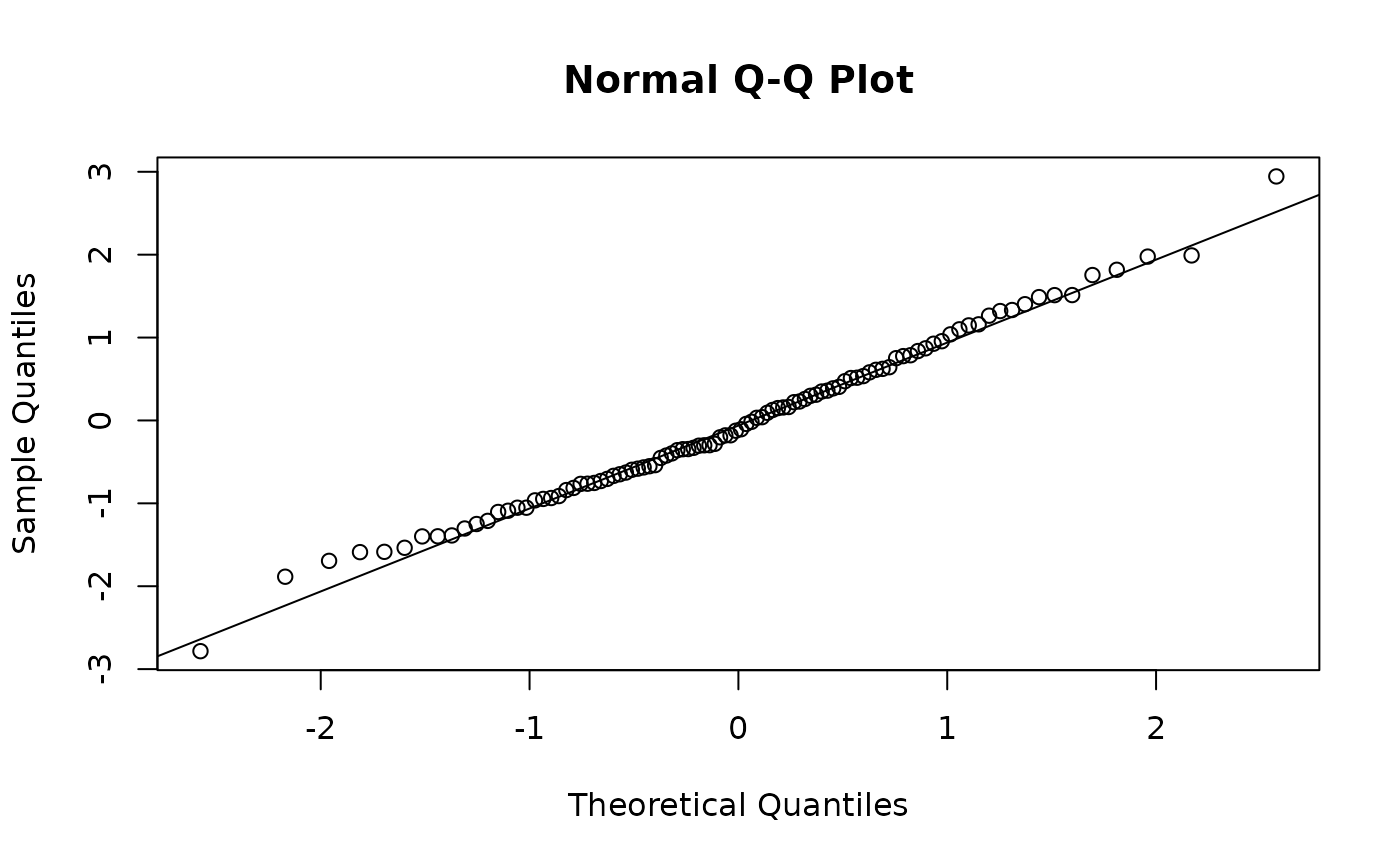
# one-step-ahead quantile residuals are standard normal under a
# correctly specified model, whatever the family. This block is
# \donttest{} because oneStepPredict() is 5.9 s of this example's
# 8.9 s, which puts the examples phase over R CMD check's 5 s
# threshold; --run-donttest still runs it.
# \donttest{
r <- residuals(fit, type = "osa")[, "Estimate"]
qqnorm(r); qqline(r)

# }