Plot case-deletion influence

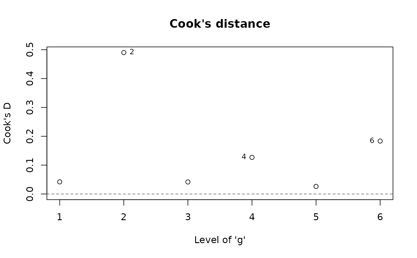
Draws the influence() result as base-graphics index plots: Cook's distances first, with the most influential cases labeled by name, then one dfbetas panel per fixed-effect coefficient. Each dfbetas panel carries the conventional +/- 2 / sqrt(n) reference band, n being the number of deleted units (Belsley, Kuh and Welsch 1980).

Usage

# S3 method for class 'frmtmb_influence'
plot(x, which = NULL, ask = NULL, labels = 3L, ...)

Arguments

x

A frmtmb_influence object from influence().

which

Panels to draw: 1 is the Cook's distance plot, 1 + j the dfbetas panel of the jth coefficient. Defaults to all of them.

ask

Pause between panels; defaults to TRUE when more than one panel goes to an interactive device, the plot.frmtmb_fit() rule.

labels

Number of extreme cases to label in each panel.

...

Passed to the underlying graphics::plot() calls.

Value

x, invisibly. Called for the plots it draws.

Details

This is deliberately NOT a car::influencePlot() counterpart: hatvalues and studentized residuals are OLS-geometry approximations to case deletion that are ill-defined for a fit whose random effects are marginalized by the Laplace approximation, and the refit-based quantities plotted here are the exact version of what those approximate.

References

Belsley, D. A., Kuh, E. and Welsch, R. E. (1980) Regression Diagnostics. Wiley.

Examples

# \donttest{
set.seed(7)
dd <- data.frame(x = rnorm(60), g = factor(rep(1:6, 10)))
dd$y <- rnorm(60, 1 + 0.5 * dd$x + rnorm(6, 0, 0.5)[dd$g], 1)
fit <- frm(bf(y ~ x + (1 | g)), family = gaussian(), data = dd)
#> Boundary (singular) fit: sd_g__Intercept is at zero. The likelihood does not change as it moves further that way, so it has no standard error (NaN in summary(), vcov() and confint()); the other standard errors are kept. lme4 reports such a fit as singular; diagnose() lists the components at the boundary
infl <- influence(fit, groups = "g")

# Cook's distances only
plot(infl, which = 1)

# }